Unified Stream and Batch Processing for Factor Development
In quantitative trading, factor discovery is the foundation of alpha generation. Whether for high-frequency crypto strategies or medium-term systematic portfolios, the ability to efficiently compute, iterate, and deploy factors directly determines research velocity and production readiness.
Traditional factor research workflows usually fall into two categories:
- Manual factor discovery , relying on researchers’ market intuition and financial expertise. While often insightful, this approach is time-consuming, difficult to scale, and limited by human cognition.
- Algorithm-driven discovery , which applies machine learning and deep learning models to automatically extract predictive patterns from market data. Neural networks, in particular, excel at capturing nonlinear relationships among price dynamics, order flow, sentiment, and macro-level variables—making them especially suitable for the highly volatile and information-dense cryptocurrency market.
However, machine-learning-based factor mining imposes extremely demanding infrastructure requirements:
- Fast access to massive historical tick or minute-level data
- Efficient batch computation for training datasets
- Low-latency streaming computation for backtesting and simulation
- Seamless integration between databases and Python-based modeling frameworks
This is precisely where DolphinDB’s unified stream-batch architecture becomes valuable.
In this article, we present a complete crypto factor research and deployment pipeline built on DolphinDB, covering:
- Minute-level factor storage design
- Batch and streaming factor computation
- Machine-learning-driven backtesting and real-time signal generation
The solution enables researchers to iterate factors offline at scale while deploying the same logic in real-time simulations—without rewriting infrastructure.
1. Designing a Minute-Level Factor Database
1.1 Storage Engine and Partitioning Strategy
Minute-level factor data exhibits three key characteristics:
- Very large volume
- Continuous appends
- Frequent time-range queries by symbol, market, and factor
To support these workloads, we recommend using DolphinDB’s TSDB storage engine together with a narrow-table schema.
The database design is summarized below (the full script is provided in the Appendix):
| Item | Configuration |
|---|---|
| Database Name | CryptocurrencyFactor |
| Storage Engine | TSDB |
| Partition Scheme | Monthly + VALUE partition by factor name |
| Partition Columns | time + factor name |
| Sort Columns | market + asset + time |
| Partition Size | ~115 MB per factor (100 assets) |
Note: If the estimated number of combinations of market and asset exceeds 1,000, it is recommended to reduce the dimension of the sort columns during database creation by adding the following parameter: sortKeyMappingFunction=[hashBucket{,3}, hashBucket{,300}].
1.2 Table Schema
The column definitions of the minute-level factor table (factor_1m) are as follows.
| Column Name | Data Type | Description |
|---|---|---|
| datetime | TIMESTAMP | Time column |
| symbol | SYMBOL | Asset for factor computation |
| market | SYMBOL | Market, such as ‘Binance-Futures’, ‘Binance-Spot’, ‘OKX-Futures’, ‘OKX-Spot’ |
| factorname | SYMBOL | Factor name |
| factorvalue | DOUBLE | Factor value |
This narrow format makes it easy to add new factors without schema changes and supports both historical analysis and real-time ingestion.
2. Factor Computation
DolphinDB ships with built-in GTJA 191 and WorldQuant 101 alpha libraries. Since most cross-sectional and fundamental-based factors are not applicable to crypto markets, we extract time-series-based factors and convert them into state functions for streaming use.
These state-aware factors are defined in stateFactors.dos. You can load the module using use or extend it with user-defined factor definitions. The complete implementation is provided in the Appendix.
Using the gtjaAlpha100 factor as an example, we demonstrate how to perform both batch and streaming computation for the same factor in DolphinDB. In stateFactors.dos, gtjaAlpha100 is defined as:
@state
def gtjaAlpha100(vol){
    return mstd(vol, 20)
}
Compared with its definition in gtja191Alpha.dos, the only difference is the addition of @state, which converts it from a regular function into a state function, enabling direct use in streaming computation.
2.1 Batch Factor Computation
Factors are computed based on minute-level OHLC data, so historical minute-level OHLC data must exist in the DolphinDB server.
Batch computation consists of three steps: retrieving historical data, generating factor computation expressions, and computing and writing results to the database. The full script is provided in the Appendix.
- Retrieve historical data from the database.
// Use the factor module
use stateFactors
go
all_data = select * from loadTable("dfs://CryptocurrencyKLine","minKLine")
factor_value_tb = loadTable("dfs://CryptocurrencyFactor", "factor_1min")
- Generate factor computation expressions.
cols_dict = {
    "vol": "volume"
}
def dict_replace_str(s, str_dict){
    for (i in str_dict.keys()){
        result = regexReplace(s, i, str_dict[i])
    }
    return result
}
use_func_call = exec name.split("::")[1]+syntax from defs() where name ilike "%stateFactors%"
funcName = func_call[:regexFind(func_call, "[()]+")]
deal_func_call = dict_replace_str(func_call, cols_dict)
select_string = stringFormat(
    "select eventTime,symbol,symbolSource,\"%W\" as factorname,
     %W as factorvalue from all_data
     context by symbol,symbolSource csort eventTime",
    funcName, deal_func_call)
Here, dict_replace_str and cols_dict are used to replace parameter names in function expressions. For example, the parameter vol corresponds to the column volume in the database, allowing you to compute factors without modifying original column names.
- Loop through all factors and append results to the database.
for (func_call in use_func_call){// func_call=use_func_call[0]
    funcName = func_call[:regexFind(func_call, "[()]+")]
    deal_func_call = dict_replace_str(func_call, cols_dict)
    select_string = stringFormat("select eventTime,symbol,symbolSource,\"%W\" as factorname, %W as factorvalue from all_data context by symbol,symbolSource csort eventTime", funcName, deal_func_call)
    result = select * from parseExpr(select_string).eval()
    factor_value_tb.append!(result)
}
2.2 Streaming Factor Computation
Factors are computed based on minute-level OHLC data, so a minute-level OHLC stream table must exist.
Streaming factor computation includes three steps: creating a factor stream table, building a narrow reactive state engine, and subscribing to upstream data streams. The full script is provided in the Appendix.
- Create a persistent stream table to store computed factor data.
// Stream table used to store factor data
output_stream = "min_factor_stream"
// Output table definition and conversion function
try{dropStreamTable(output_stream)}catch(ex){}
temp = streamTable(1:0, ["datetime","symbol","market","factorname","factorvalue"],
        ["TIMESTAMP","SYMBOL","SYMBOL","SYMBOL","DOUBLE"])
enableTableShareAndCachePurge(temp, output_stream, 10000000)
def output_handler(msg, output_stream){
    if (count(msg) == 0){return}
    cols = msg.columnNames()[2 0 1 3 4]
    tb = objByName(output_stream)
    tb.append!(<select _$$cols from msg>.eval())
}
//Used as a placeholder for output table in the engine with no actual effect.
try{dropStreamTable("output_tmp")}catch(ex){}
share streamTable(1:0, ["symbol","market","datetime","factorname","factorvalue"],
        ["SYMBOL","SYMBOL","TIMESTAMP","SYMBOL","DOUBLE"]) as output_tmp
Before building the reactive state engine that returns a table in narrow format, the output table and output handler must be created. The above code defines output_handler and two stream tables (output_stream and output_tmp). The output_handler function will serve as the outputHandler parameter for the engine. After setting this parameter, the results will no longer be written to the output table, but instead, output_handler will process the results. Therefore, the actual result writing happens at line 12 of the code. output_tmp is used as a placeholder, and after the engine is created, this stream table can be deleted.
- Build the narrow reactive state engine.
// List of required factor function names
func_table = select * from defs() where name ilike "%stateFactors%"
factor_fuc_name = func_table["name"].split("::")[1]
// List of factor metric computation meta-code
factor = [<eventTime>]
factor_fuc_syntax = parseExpr(func_table["name"] + func_table["syntax"])
factor.appendTuple!(factor_fuc_syntax)
engine_name = "cryto_cal_min_factor_stream"
// Try to drop the existing stream engine, if any
try { dropStreamEngine(engine_name) } catch (ex) {}
// Create the narrow reactive state engine
engine = createNarrowReactiveStateEngine(
    name=engine_name,
    keyColumn=["symbol", "symbolSource"], // Grouping columns
    metrics=factor, // Factor computation meta-code
    metricNames=factor_fuc_name, // Factor name
    dummyTable=table(1:0, ["eventTime", "collectionTime", "symbolSource", "symbol", "open", "high", "low", "close", "vol", "numberOfTrades", "quoteVolume", "takerBuyBase", "takerBuyQuote", "volCcy"], ["TIMESTAMP", "TIMESTAMP", "SYMBOL", "SYMBOL", "DOUBLE", "DOUBLE", "DOUBLE", "DOUBLE", "DOUBLE", "INT", "DOUBLE", "DOUBLE", "DOUBLE", "DOUBLE"]),
    outputHandler=output_handler{, output_stream},
    outputTable=objByName("output_tmp"),
    msgAsTable=true
)
try { dropStreamTable("output_tmp") } catch (ex) {}
To add custom factors, you only need to append factor names and computation logic to factor_fuc_name and factor.
- Subscribe to upstream data streams.
For example, subscribe to Cryptocurrency_minKLineST, the minute-level OHLC stream table.
input_stream = 'Cryptocurrency_minKLineST'
try{unsubscribeTable(,input_stream, "cal_min_factors")}catch(ex){}
subscribeTable(,input_stream, "cal_min_factors", getPersistenceMeta(objByName(input_stream))["memoryOffset"], engine, msgAsTable=true, throttle=1, batchSize=10)
3. Model Training and Real-Time Signal Generation
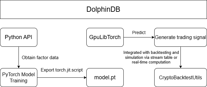
After factor computation and storage, machine learning models are trained and applied to backtesting and simulation for generating trading signals. The workflow consists of four steps:
- factor data retrieval and preprocessing;
- factor model training in Python;
- factor model export;
- trading signal prediction within DolphinDB combined with the backtesting and simulation framework. The fourth step supports both historical and real-time signal generation. The overall workflow is illustrated in the following figure.
3.1 Data Retrieval and Preprocessing
Historically computed factor data is stored in dfs://CryptocurrencyFactor, currently containing only 1-minute factors, with more frequencies to be added in the future. To simplify factor data retrieval and standardization in a Python client via the DolphinDB API, preprocessing is encapsulated in the Python class FactorDataloader. All preprocessing is executed on the DolphinDB server, and the Python client only receives the processed data.
FactorDataloader provides preprocessing support for LSTM, XGBoost, and Transformer models. Example:
from DataPre import FactorDataloader
ddb_connect = ddb.session("ip", port)
t = FactorDataloader(
    db_connect=ddb_connect,
    symbol="BTCUSDT",
    start_date="2024.03.01",
    end_date="2024.03.02",
    factor_name=["gtjaAlpha2"],
    market="Binance-Futures",
)
train_loader, test_loader = t.get_LSTM_dataloader(10, 0.2, 32)
train_loader, test_loader = t.get_xgboost_data(0.2)
train_loader, test_loader = t.get_transformer_data(1440, 0.2, 32)
3.2 Python Model Training
The DolphinDB’s GpuLibTorch plugin allows you to load and run the TorchScript model exported from Python, combining DolphinDB’s data processing capabilities with PyTorch’s deep learning functionality. You can run the following functions to install and load the GpuLibTorch plugin.
login("admin", "123456")
listRemotePlugins()
installPlugin("GpuLibTorch")
loadPlugin("GpuLibTorch")
The plugin does not support training models within DolphinDB, so training must be performed in a Python environment. A generic training and evaluation framework for three-class classification tasks is implemented in Models.py, supporting LSTM and Transformer models. The related functions are as follows:
# Functions
evaluate_classify_model(model, test_loader, device=torch.device("cuda" if torch.cuda.is_available() else "cpu"))
train_model(
    model,
    criterion,
    optimizer,
    num_epochs: int,
    train_loader,
    test_loader,
    device=torch.device("cuda" if torch.cuda.is_available() else "cpu"),
    per_epoch_show: int = 20,
)
# Usage
# Model training
criterion = nn.CrossEntropyLoss()
optimizer = optim.Adam(model.parameters(), lr=0.001, weight_decay=1e-5)
trained_model = train_model(
    model=model,
    criterion=criterion,
    optimizer=optimizer,
    num_epochs=100,
    train_loader=train_loader,
    test_loader=test_loader,
)
# Model evaluation
accuracy, preds, targets = evaluate_classify_model(trained_model, test_loader)
3.3 Model Export
After training in Python, the model needs to be exported as a model.pth file for prediction in DolphinDB. Models exported using torch.jit.trace may cause an error when loading in DolphinDB due to hidden layer tensors and input tensors not being on the same device. Therefore, we recommend that you use torch.jit.script to export the model file.
torch.jit.script(model).save("model.pth")
3.4 Model Prediction and Backtesting/Simulation
Historical Computation Method
After obtaining the model, predictions can be made on upstream factor data using the GpuLibtorch plugin to generate trading signals for backtesting. This method requires pre-computed future signals and is suitable for backtesting only. For real-time simulation, the real-time computation method discussed later should be used.
table_name = "factor_predict_result"
try{
    undef(table_name, SHARED)
    print(table_name+" exists, stream table cleared")
} catch(ex) {
    print(table_name+" does not exist, environment cleaned")
}
share(table(100000: 0, `datetime`signal, [TIMESTAMP, INT]), table_name)
model = GpuLibTorch::load(model_file)
predict_result = GpuLibTorch::predict(model, data_input)
The above code creates a stream table named factor_predict_result to store the pre-computed signals for easy retrieval during backtesting. As shown in lines 9-10, you can load the trained model using GpuLibTorch and input pre-processed data (data_input) to get the model output (predict_result). The results are then inserted into the factor_predict_result stream table. The preprocessing of data_input is detailed in the DataPre.py script provided in the Appendix.
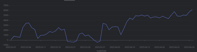
After obtaining the trading signal stream table factor_predict_result, it can be used in the event callback function for backtesting. The following example generates trading signals for BTCUSDT from 2025.03.01 to 2025.05.01 using an LSTM model, as shown in line 3. The callback function performs buy and sell operations based on the signal, as shown in lines 11 and 17. The full script is in the Appendix.
def onBar(mutable context, msg, indicator){
    //...
    singal_t = objByName("factor_predict_result")
    for(isymbol in msg.keys()){
        source = msg[isymbol]["symbolSource"]
        lastPrice = msg[isymbol]["close"]
        tdt = msg[isymbol]["tradeTime"]
        signal = exec signal from singal_t where datetime=tdt
        signal = signal[0]
        if (signal==int(NULL)){break}
        if (signal==0){
            // Sell
            qty = Backtest::getPosition(context["engine"], isymbol, "futures").longPosition
            if (qty > 0){
                Backtest::submitOrder(context["engine"], (isymbol, source, context["tradeTime"], 0, lastPrice, 0, 1000000, qty, 3, 0, 0, context["tradeTime"].temporalAdd(1m)), "sell", 0, "futures")
            }
        } else if (signal==2){
            // Buy
            Backtest::submitOrder(context["engine"], (isymbol, source, context["tradeTime"], 5, lastPrice, 0, 1000000, 0.001, 1, 0, 0, context["tradeTime"].temporalAdd(1m)), "buy", 0, "futures")
        }
    }
}
After the backtest is completed, the daily realized profit and loss curve can be plotted as shown in the following figure:
result = select * from day where accountType="futures"
plot((double(result["realizedPnl"])), result["tradeDate"])
Real-time computation method
In addition to pre-computing trading signals for backtesting based on historical data, you can also simulate real-time trading by computing real-time factors and generating trading signals using a pre-trained model. This method is suitable for both historical market backtesting and simulated trading.
Below is the core code for a minute-level backtest demo that uses the gtjaAlpha94 and gtjaAlpha50 alpha factors for prediction. Since the factor computation functions in the built-in factor library of DolphinDB are not state functions, you need to use the factor computation functions that have been converted to state functions in the stateFactors module (see the previous section for module description).
- Pre-load the required model using a shared dictionary.
// Initialize the model through a shared dictionary
model_dir = "/home/customer/model_config/test_LSTM.pth"
model = GpuLibTorch::load(model_dir)
GpuLibTorch::setDevice(model, "CUDA")
try{undef("test_ml_model", SHARED)}catch(ex){}
test_ml_model = syncDict(STRING, ANY, "test_ml_model")
go;
test_ml_model["model"] = model
This avoids reloading the model during subsequent computation. After loading the model, the GpuLibTorch::setDevice function must be called to specify the computing device for prediction. Otherwise, the default CPU will be used.
- Subscribe to signals in the
initializefunction to compute metrics.
def gen_signal(factor1, factor2){
    model = objByName("test_ml_model")["model"]
    data_input = matrix(zscore(factor1).nullFill!(0), zscore(factor2)).nullFill!(0).float()
    data_input = tensor(array(ANY).append!(data_input))
    x = GpuLibTorch::predict(model, data_input)[0]
    signal = imax(1/(1+exp(x*-1)))
    return signal
}
def initialize(mutable context){
    print("initialize load model")
    // Metric subscription
    indicator_dict = dict(STRING, ANY)
    indicator_dict["signal"] = <moving(gen_signal, (gtjaAlpha94(close.double(), volume.double()), gtjaAlpha50(high.double(), low.double())), 20)>

    Backtest::subscribeIndicator(context["engine"], "kline", indicator_dict, "futures")
}
By defining the meta-code in the initialize function, the backtesting engine can compute factor data in real time during backtesting and simulation. The corresponding model can be called in the signal computation function to generate signals. The event callback functions then obtain the trading signals through the indicator parameter. Here’s a usage example for the onBar callback function:
def onBar(mutable context, msg, indicator){
    //...
    one_msg = msg[isymbol]
    one_indicator = indicator[isymbol]
    signal = one_indicator["signal"]
    tdt = one_msg["tradeTime"]
    if (signal == int(NULL)){continue}
    if (signal == 0){
        // Sell
        qty = Backtest::getPosition(context["engine"], isymbol, "futures").longPosition
        if (qty > 0){
            Backtest::submitOrder(context["engine"], (isymbol, source, context["tradeTime"], 0, lastPrice, 0, 1000000, qty, 3, 0, 0, context["tradeTime"].temporalAdd(1m)), "sell", 0, "futures")
        }
    }else if (signal == 2){
        // Buy
        Backtest::submitOrder(context["engine"], (isymbol, source, context["tradeTime"], 5, lastPrice, 0, 1000000, 0.001, 1, 0, 0, context["tradeTime"].temporalAdd(1m)), "buy", 0, "futures")
    }
}
In the above onBar callback function, you can obtain the real-time computed results of the signal generation function, which are subscribed to in the initialize function, through the indicator parameter, and then open or close positions based on the corresponding signals. The full script is provided in the Appendix.
Conclusion
In this article, we’ve shown how DolphinDB’s unified stream and batch processing architecture enables efficient factor discovery, machine learning model training, and real-time signal generation for cryptocurrency markets. By combining fast data processing with seamless integration to Python, DolphinDB empowers researchers to iterate on factors and deploy them quickly in both offline and live environments.
This architecture provides a strong foundation for building scalable, real-time quantitative strategies across asset classes, helping teams stay ahead in the competitive world of algorithmic trading. With DolphinDB, you can accelerate your research, deploy faster, and make better decisions in ever-changing markets.
Appendix
- State factor expression module: stateFactors.dos
- Daily batch factor computation: calfactor.dos
- Streaming factor computation: real_time_cal_factor.dos
- Factor database and table creation: createFactorDatabaseTable.dos
- Python environment dependencies: requirements.txt
- Training examples for different models: LSTM_main.py, xgboost_main.py, LSTM_and_xgboost_main.py, transformer_main.py
- Backtesting demo based on stream tables: main.py, factorStrategy.dos, model.pth
- Backtesting demo based on real-time computation: demo.dos, test_LSTM.pth, test_LSTM_cpu.pth