How to Build 1-Minute OHLC Bars from Non-Uniform Market Snapshot Data

In financial markets, every price tells a story — but raw snapshot data, arriving every few seconds in irregular bursts, tells it in a format most systems weren’t built to read directly. Before you can do anything useful with it, you need to reshape it: turn thousands of uneven slices into clean, evenly-spaced OHLC bars that charting tools, backtesting engines, and trading algorithms actually understand.

This article walks through exactly that transformation, using DolphinDB as the computing layer. We’ll cover both the batch path (historical data, processed in parallel) and the streaming path (real-time data, processed with sub-millisecond latency), with the same core logic running in both.

The Data We’re Working With

Level-1 and Level-2 snapshot data for equity markets (SSE, SZSE, and BSE) is published at roughly 3-second intervals — but the intervals aren’t uniform. An actively traded stock might have dense, near-continuous snapshots; an illiquid fund might have gaps of 10 seconds or more. The result, across roughly 6,000+ symbols, is around 24 million rows of data per trading day.

The trading session itself has a particular structure worth noting:

• Opening call auction: 09:15:00–09:25:00
• Continuous auction: 09:30:00–11:30:00
• Continuous auction: 13:00:00–14:57:00
• Closing call auction: 14:57:00–15:00:00

The snapshot table carries all the fields you’d expect — LastPrice, HighPrice, LowPrice, TotalVolumeTrade, TotalValueTrade — along with cumulative daily counters and a few fund-specific fields like IOPV.

Why Snapshot-to-OHLC Isn’t Trivial

At first glance it seems straightforward: group by symbol and minute, take first/last/max/min, sum up volume. But several edge cases make this harder than it looks.

High and Low prices are cumulative within the day. The HighPrice field in each snapshot is the day's high at that moment, not the high of the last 3 seconds. If no new high was set during a particular 1-minute window, the value doesn't change between snapshots — it just carries forward. This means you can't simply take max(HighPrice) across a window and call it the bar's high. You need to detect whether the intraday high actually changed during that window, and only then use max(HighPrice); otherwise, use max(LastPrice).

The same logic applies inversely to low prices.

Volume and trade counts are also cumulative. You need to calculate the increment between adjacent snapshots before aggregating.

Some windows will be empty. Inactive instruments may go minutes at a time with no new trades, even though snapshots keep arriving. For those windows, the OHLC values should carry forward from the previous bar — not be filled with zeros.

The opening call auction needs special handling. Data from the 09:25–09:30 window (call auction) belongs to the first 1-minute bar, whose output timestamp is 09:30:00. The calculation window for that bar is effectively [09:25:00, 09:31:00).

Part 1: Generating OHLC Bars from Historical Snapshot Data

Step 1: Deploy the Test Environment

• Deploy the DolphinDB server in standalone mode: Standalone Deployment and Upgrade.
• Download the test data and upload it to the server directory of your DolphinDB server.

Step 2: Create the Database and Partitioned Table

The database and partitioned table creation code below applies when Level-2 snapshot data for stocks and funds from both the SSE and SZSE is stored in the same table. For more information about creating databases and partitioned tables, see Best Practices for Financial Data Storage.

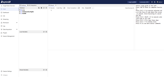
Paste the following code into the web interface, select the code you want to run, and click Execute (shortcut: Ctrl+E).

• Open the web interface as instructed in the deployment tutorial. After logging in, run the test code as follows. The default admin account is admin with the password 123456.

//Create the database
create database "dfs://snapshotDB"
partitioned by VALUE(2020.01.01..2021.01.01), HASH([SYMBOL, 50])
engine='TSDB'
//Create the partitioned table
create table "dfs://snapshotDB"."snapshotTB"(
    Market SYMBOL
    TradeTime TIMESTAMP
    MDStreamID SYMBOL
    SecurityID SYMBOL
    SecurityIDSource SYMBOL
    TradingPhaseCode SYMBOL
    ImageStatus INT
    PreCloPrice DOUBLE
    NumTrades LONG
    TotalVolumeTrade LONG
    TotalValueTrade DOUBLE
    LastPrice DOUBLE
    OpenPrice DOUBLE
    HighPrice DOUBLE
    LowPrice DOUBLE
    ClosePrice DOUBLE
    DifPrice1 DOUBLE
    DifPrice2 DOUBLE
    PE1 DOUBLE
    PE2 DOUBLE
    PreCloseIOPV DOUBLE
    IOPV DOUBLE
    TotalBidQty LONG
    WeightedAvgBidPx DOUBLE
    AltWAvgBidPri DOUBLE
    TotalOfferQty LONG
    WeightedAvgOfferPx DOUBLE
    AltWAvgAskPri DOUBLE
    UpLimitPx DOUBLE
    DownLimitPx DOUBLE
    OpenInt INT
    OptPremiumRatio DOUBLE
    OfferPrice DOUBLE[]
    BidPrice DOUBLE[]
    OfferOrderQty LONG[]
    BidOrderQty LONG[]
    BidNumOrders INT[]
    OfferNumOrders INT[]
    ETFBuyNumber INT
    ETFBuyAmount LONG
    ETFBuyMoney DOUBLE
    ETFSellNumber INT
    ETFSellAmount LONG
    ETFSellMoney DOUBLE
    YieldToMatu DOUBLE
    TotWarExNum DOUBLE
    WithdrawBuyNumber INT
    WithdrawBuyAmount LONG
    WithdrawBuyMoney DOUBLE
    WithdrawSellNumber INT
    WithdrawSellAmount LONG
    WithdrawSellMoney DOUBLE
    TotalBidNumber INT
    TotalOfferNumber INT
    MaxBidDur INT
    MaxSellDur INT
    BidNum INT
    SellNum INT
    LocalTime TIME
    SeqNo INT
    OfferOrders LONG[]
    BidOrders LONG[]
)
partitioned by TradeTime, SecurityID,
sortColumns=[`Market,`SecurityID,`TradeTime],
keepDuplicates=ALL

If the code runs without errors, it has executed successfully. You can then run the following code to view the partitioned table schema:

loadTable("dfs://snapshotDB", "snapshotTB").schema().colDefs

The output:

Step 3: Import the Test CSV Data

Run the following code to import the test CSV data. Note that before running the following code, upload the test data file testData.csv to the server directory of your DolphinDB server. You can also upload the CSV file to a user-defined path, such as /data/testData.csv. In that case, set filename="/data/testData.csv" in the loadTextEx function in the following code.

tmp = loadTable("dfs://snapshotDB", "snapshotTB").schema().colDefs
schemaTB = table(tmp.name as name, tmp.typeString as type)
loadTextEx(dbHandle=database("dfs://snapshotDB"), tableName="snapshotTB", partitionColumns=`TradeDate`SecurityID, filename="./testData.csv", schema=schemaTB)

After successful import, run the following code to load the first 10 rows into memory to preview the data:

data = select top 10 * from loadTable("dfs://snapshotDB", "snapshotTB")

The output:

Step 4: Define User-Defined Functions to Calculate High and Low Prices

Run the following code to define user-defined functions in the current session. You can then call the high and low functions in subsequent operations within the same session:

defg high(DeltasHighPrice, HighPrice, LastPrice){
 if(sum(DeltasHighPrice)>0.000001){
  return max(HighPrice)
 }
 else{
  return max(LastPrice)
 }
}

defg low(DeltasLowPrice, LowPrice, LastPrice){
 sumDeltas = sum(DeltasLowPrice)
 if(sumDeltas<-0.000001 and sumDeltas!=NULL){
  return min(iif(LowPrice==0.0, NULL, LowPrice))
 }
 else{
  return min(LastPrice)
 }
}

Step 5: Load a Small Sample into Memory for Debugging

To make it easier to verify that the code works well during debugging, you can first load a small amount of data into memory, which also makes it easier to debug more complex business logic later.

Run the following code to load one day’s data for two symbols into memory and assign it to the table snapshotTB. In the subsequent code, you can reference the snapshotTB for debugging:

snapshotTB = select TradeTime, SecurityID, OpenPrice,
   PreCloPrice, HighPrice, LowPrice,
   LastPrice, PreCloseIOPV, IOPV,
   TotalVolumeTrade, TotalValueTrade, NumTrades,
   UpLimitPx, DownLimitPx
  from loadTable("dfs://snapshotDB", "snapshotTB")
  where TradeTime.date()=2023.02.01, SecurityID in `888888`999999

Step 6: Process the Raw Snapshot Data

Run the following code to process the raw snapshot data. The main transformations are as follows:

• Include the data from 09:25:00 to 09:30:00 in the first OHLC bar: [09:30:00, 09:31:00].
• Calculate the changes in the high and low prices between two adjacent snapshots of the same stock or fund.
• Calculate the increments in trading volume, trading value, and trade count between two adjacent snapshots of the same stock or fund.

tempTB1 = select TradeTime.date() as TradeDate,
   iif(TradeTime.time()<=09:30:00.000, 09:30:00.000, TradeTime.time()) as TradeTime,
   SecurityID,
   OpenPrice,
   PreCloPrice,
   HighPrice,
   LowPrice,
   LastPrice,
   PreCloseIOPV,
   IOPV,
   UpLimitPx,
   DownLimitPx,
   iif(deltas(HighPrice)>0.000001, 1, 0) as DeltasHighPrice,
   iif(abs(deltas(LowPrice))>0.000001, -1, 0) as DeltasLowPrice,
   iif(deltas(TotalVolumeTrade)==NULL, TotalVolumeTrade, deltas(TotalVolumeTrade)) as DeltasVolume,
   iif(deltas(TotalValueTrade)==NULL, TotalValueTrade, deltas(TotalValueTrade)) as DeltasTurnover,
   iif(deltas(NumTrades)==NULL, NumTrades, deltas(NumTrades)) as DeltasTradesCount
  from snapshotTB
  where TradeTime.time()>=09:25:00.000
  context by SecurityID

Step 7: Perform Aggregation with a 1-Minute Window and 1-Minute Step

Run the following code to perform rolling-window aggregation on the processed snapshot data using a 1-minute window and a 1-minute step. The key steps are as follows:

• Call the user-defined functions high and low to calculate the high and low prices of the OHLC bar.
• FirstBarChangeRate indicates the change between the first snapshot with a nonzero latest price and the latest snapshot with a nonzero latest price within the current 1-minute calculation window. It is used to calculate the price change for the opening OHLC bar.
• This downsampling step calls the DolphinDB built-in function interval. At this stage, if snapshot data is missing from an intraday calculation window, the code fills the values with 0. In a later step, it further processes OHLC bars with all values 0.

tempTB2 = select firstNot(LastPrice, 0) as OpenPrice,
   high(DeltasHighPrice, HighPrice, LastPrice) as HighPrice,
   low(DeltasLowPrice, LowPrice, LastPrice) as LowPrice,
   last(LastPrice) as ClosePrice,
   sum(DeltasVolume) as Volume,
   sum(DeltasTurnover) as Turnover,
   sum(DeltasTradesCount) as TradesCount,
   last(PreCloPrice) as PreClosePrice,
   last(PreCloseIOPV) as PreCloseIOPV,
   last(IOPV) as IOPV,
   last(UpLimitPx) as UpLimitPx,
   last(DownLimitPx) as DownLimitPx,
   lastNot(LastPrice, 0)\firstNot(LastPrice, 0)-1 as FirstBarChangeRate 
  from tempTB1
  group by SecurityID, TradeDate, interval(X=TradeTime, duration=60s, label='left', fill=0) as TradeTime

Step 8: Align 240 Daily OHLC Bars

In this example, a total of 240 OHLC bars are generated:

• The output time of the first OHLC bar is 09:30:00, and its calculation window is [09:25:00, 09:31:00).
• The full output includes the bars at 11:30:00, 14:57:00, and 15:00:00, but excludes those at 14:58:00 and 14:59:00.

If you need to customize the output rules — for example, to output OHLC bars for the two special periods 14:58:00 and 14:59:00 — you can modify the following code.

codes = select distinct(SecurityID) as SecurityID from tempTB2 order by SecurityID
allTime = table((take(0..120, 121)*60*1000+09:30:00.000).join(take(0..117, 118)*60*1000+13:00:00.000).join(15:00:00.000) as TradeTime)
tempTB3 = cj(codes, allTime)

Step 9: Fill Calculation Windows with Missing Snapshot Data

Run the following code to process the aligned 240 daily OHLC bars data as follows and retrieve the final result:

• For calculation windows with no intraday trades, fill the values of OpenPrice, HighPrice, LowPrice, and ClosePrice with the ClosePrice of the previous OHLC bar.
• For calculation windows with no intraday trades, fill the values of PreClosePrice, PreCloseIOPV, IOPV, UpLimitPx, and DownLimitPx with the corresponding values from the previous OHLC bar.
• For the OHLC bar after the open, the price change equals the change between the latest price in the last snapshot and the latest price in the first snapshot within the [09:25:00, 09:31:00) calculation window

result = select SecurityID,
  concatDateTime(TradeDate, TradeTime) as TradeTime,
  iif(OpenPrice==0.0 and PreClosePrice==0.0, cumlastNot(ClosePrice, 0.0), OpenPrice) as OpenPrice,
  iif(HighPrice==0.0 and PreClosePrice==0.0, cumlastNot(ClosePrice, 0.0), HighPrice) as HighPrice,
  iif(LowPrice==0.0 and PreClosePrice==0.0, cumlastNot(ClosePrice, 0.0), LowPrice) as LowPrice,
  iif(ClosePrice==0.0 and PreClosePrice==0.0, cumlastNot(ClosePrice, 0.0), ClosePrice) as ClosePrice,
  Volume,
  Turnover,
  TradesCount,
  iif(PreClosePrice==0.0, cumlastNot(PreClosePrice, 0.0), PreClosePrice) as PreClosePrice,
  iif(PreCloseIOPV==0.0 and PreClosePrice==0.0, cumlastNot(PreCloseIOPV, 0.0), PreCloseIOPV).nullFill(0.0) as PreCloseIOPV,
  iif(IOPV==0.0 and PreCloseIOPV==0.0, cumlastNot(IOPV, 0.0), IOPV).nullFill(0.0) as IOPV,
  iif(UpLimitPx==0.0, cumlastNot(UpLimitPx, 0.0), UpLimitPx).nullFill(0.0) as UpLimitPx,
  iif(DownLimitPx==0.0, cumlastNot(DownLimitPx, 0.0), DownLimitPx).nullFill(0.0) as DownLimitPx,
  iif( time(TradeTime)==09:30:00.000,
   iif(FirstBarChangeRate!=NULL, FirstBarChangeRate, 0.0),
   iif(ratios(ClosePrice)!=NULL and ClosePrice!=0.0, ratios(ClosePrice)-1, 0.0)) as ChangeRate
 from lj(tempTB3, tempTB2, `TradeTime`SecurityID)
 context by SecurityID

The output:

Step 10: Encapsulate the Parallel Computing Code

After completing the first nine steps, you can already generate OHLC bars from a small volume of snapshot data. To process massive volumes of historical market data, you still need to encapsulate the code further so it can run in parallel.

First, run the following code to clear all temporary in-memory variables in the current session:

undef all

Then run the following code to define the functions for parallel computing:

defg high(DeltasHighPrice, HighPrice, LastPrice){
 if(sum(DeltasHighPrice)>0.000001){
  return max(HighPrice)
 }
 else{
  return max(LastPrice)
 }
}

defg low(DeltasLowPrice, LowPrice, LastPrice){
 sumDeltas = sum(DeltasLowPrice)
 if(sumDeltas<-0.000001 and sumDeltas!=NULL){
  return min(iif(LowPrice==0.0, NULL, LowPrice))
 }
 else{
  return min(LastPrice)
 }
}

def calOHLCBaseOnSnapshotMapFuc(snapshotTB){
 //Processing the original snapshot market table for calculating OHLC
 tempTB1 = select TradeTime.date() as TradeDate,
    iif(TradeTime.time()<=09:30:00.000, 09:30:00.000, TradeTime.time()) as TradeTime,
    SecurityID,
    OpenPrice,
    PreCloPrice,
    HighPrice,
    LowPrice,
    LastPrice,
    PreCloseIOPV,
    IOPV,
    UpLimitPx,
    DownLimitPx,
    iif(deltas(HighPrice)>0.000001, 1, 0) as DeltasHighPrice,
    iif(abs(deltas(LowPrice))>0.000001, -1, 0) as DeltasLowPrice,
    iif(deltas(TotalVolumeTrade)==NULL, TotalVolumeTrade, deltas(TotalVolumeTrade)) as DeltasVolume,
    iif(deltas(TotalValueTrade)==NULL, TotalValueTrade, deltas(TotalValueTrade)) as DeltasTurnover,
    iif(deltas(NumTrades)==NULL, NumTrades, deltas(NumTrades)) as DeltasTradesCount
   from snapshotTB
   where TradeTime.time()>=09:25:00.000
   context by SecurityID
 //Aggregate Calculating: temporary 1-minute OHLC table
 tempTB2 = select firstNot(LastPrice, 0.0) as OpenPrice,
    high(DeltasHighPrice, HighPrice, LastPrice) as HighPrice,
    low(DeltasLowPrice, LowPrice, LastPrice) as LowPrice,
    last(LastPrice) as ClosePrice,
    sum(DeltasVolume) as Volume,
    sum(DeltasTurnover) as Turnover,
    sum(DeltasTradesCount) as TradesCount,
    last(PreCloPrice) as PreClosePrice,
    last(PreCloseIOPV) as PreCloseIOPV,
    last(IOPV) as IOPV,
    last(UpLimitPx) as UpLimitPx,
    last(DownLimitPx) as DownLimitPx,
    lastNot(LastPrice, 0.0)\firstNot(LastPrice, 0.0)-1 as FirstBarChangeRate 
  from tempTB1
  group by SecurityID, TradeDate, interval(X=TradeTime, duration=60s, label='left', fill=0) as TradeTime
 //240 bars per day
 codes = select distinct(SecurityID) as SecurityID from tempTB2 order by SecurityID
 allTime = table((take(0..120, 121)*60*1000+09:30:00.000).join(take(0..117, 118)*60*1000+13:00:00.000).join(15:00:00.000) as TradeTime)
 tempTB3 = cj(codes, allTime)
 //Processing missing data calculation window, excluding opening
 result = select SecurityID,
   concatDateTime(TradeDate, TradeTime) as TradeTime,
   iif(OpenPrice==0.0 and PreClosePrice==0.0, cumlastNot(ClosePrice, 0.0), OpenPrice) as OpenPrice,
   iif(HighPrice==0.0 and PreClosePrice==0.0, cumlastNot(ClosePrice, 0.0), HighPrice) as HighPrice,
   iif(LowPrice==0.0 and PreClosePrice==0.0, cumlastNot(ClosePrice, 0.0), LowPrice) as LowPrice,
   iif(ClosePrice==0.0 and PreClosePrice==0.0, cumlastNot(ClosePrice, 0.0), ClosePrice) as ClosePrice,
   Volume,
   Turnover,
   TradesCount,
   iif(PreClosePrice==0.0, cumlastNot(PreClosePrice, 0.0), PreClosePrice) as PreClosePrice,
   iif(PreCloseIOPV==0.0 and PreClosePrice==0.0, cumlastNot(PreCloseIOPV, 0.0), PreCloseIOPV).nullFill(0.0) as PreCloseIOPV,
   iif(IOPV==0.0 and PreCloseIOPV==0.0, cumlastNot(IOPV, 0.0), IOPV).nullFill(0.0) as IOPV,
   iif(UpLimitPx==0.0, cumlastNot(UpLimitPx, 0.0), UpLimitPx).nullFill(0.0) as UpLimitPx,
   iif(DownLimitPx==0.0, cumlastNot(DownLimitPx, 0.0), DownLimitPx).nullFill(0.0) as DownLimitPx,
   iif( time(TradeTime)==09:30:00.000,
    iif(FirstBarChangeRate!=NULL, FirstBarChangeRate, 0.0),
    iif(ratios(ClosePrice)!=NULL and ClosePrice!=0.0, ratios(ClosePrice)-1, 0.0)) as ChangeRate
  from lj(tempTB3, tempTB2, `TradeTime`SecurityID)
  context by SecurityID
 return result
}

def calOHLCBaseOnSnapshot(calStartDate, calEndDate, dbName, tbName){
 //Generate data source: If SQL only contains the required columns for calculation, it can improve calculation efficiency
 dataSource = sqlDS(< select TradeTime, SecurityID, OpenPrice,
     PreCloPrice, HighPrice, LowPrice,
     LastPrice, PreCloseIOPV, IOPV,
     TotalVolumeTrade, TotalValueTrade, NumTrades,
     UpLimitPx, DownLimitPx
    from loadTable(dbName, tbName)
    where TradeTime.date()>=calStartDate, TradeTime.date()<=calEndDate>)
 result = mr(ds=dataSource, mapFunc=calOHLCBaseOnSnapshotMapFuc, finalFunc=unionAll{,false}, parallel=true)

Finally, run the following code to generate 1-minute OHLC bars in parallel from one day’s full snapshot data for the SSE and SZSE.

calStartDate = 2023.02.01
calEndDate = 2023.02.01
dbName = "dfs://snapshotDB"
tbName = "snapshotTB"
oneDayResult = calOHLCBaseOnSnapshot(calStartDate, calEndDate, dbName, tbName)

Step 11: Store 1-Minute OHLC Bars Data

Run the following code to create the database and partitioned table to store 1-minute OHLC bars before storing data for the first time:

def createStockFundOHLCDfsTB(dbName="dfs://stockFundOHLC", tbName="stockFundOHLC"){
 if(existsDatabase(dbUrl=dbName)){
  print(dbName + " has been created !")
  print(tbName + " has been created !")
 }
 else{
  db = database(dbName, VALUE, 2021.01.01..2021.12.31)
  print(dbName + " created successfully.")
  colNames = `SecurityID`TradeTime`OpenPrice`HighPrice`LowPrice`ClosePrice`Volume`Turnover`TradesCount`PreClosePrice`PreCloseIOPV`IOPV`UpLimitPx`DownLimitPx`ChangeRate
  colTypes = [SYMBOL, TIMESTAMP, DOUBLE, DOUBLE, DOUBLE, DOUBLE, LONG, DOUBLE, INT, DOUBLE, DOUBLE, DOUBLE, DOUBLE, DOUBLE, DOUBLE]
  schemaTable = table(1:0, colNames, colTypes)
  db.createPartitionedTable(table=schemaTable, tableName=tbName, partitionColumns=`TradeTime)
  print(tbName + " created successfully.")
 }
 return loadTable(dbName, tbName).schema().colDefs
}
dbName = "dfs://stockFundOHLC"
tbName = "stockFundOHLC"
createStockFundOHLCDfsTB(dbName, tbName)

Run the following code to persist the results from memory into the partitioned table:

loadTable("dfs://stockFundOHLC", "stockFundOHLC").append!(oneDayResult)

Load the first 10 rows into memory to preview:

data = select top 10 * from loadTable("dfs://stockFundOHLC", "stockFundOHLC")

The output:

Benchmark results on 16 CPU cores (Intel Xeon Gold 5220R @ 2.20 GHz):

Part 2: Generating OHLC Bars from Real-Time Snapshot Data

The streaming architecture chains three engines together, each with a focused responsibility:

Press enter or click to view image in full size

Next, we will explain in detail how to write the code in DolphinDB to generate OHLC bars from real-time snapshot data. This tutorial does not cover the basic concepts of DolphinDB’s streaming feature. For more information, see the official tutorial: Stream for DolphinDB.

Define Functions to Create Stream Tables

Run the following code to define the functions to create the stream tables:

def getMDLSnapshotTB(tableCapacity=1000000){
 colNames = `Market`TradeTime`MDStreamID`SecurityID`SecurityIDSource`TradingPhaseCode`ImageStatus`PreCloPrice`NumTrades`TotalVolumeTrade`TotalValueTrade`LastPrice`OpenPrice`HighPrice`LowPrice`ClosePrice`DifPrice1`DifPrice2`PE1`PE2`PreCloseIOPV`IOPV`TotalBidQty`WeightedAvgBidPx`AltWAvgBidPri`TotalOfferQty`WeightedAvgOfferPx`AltWAvgAskPri`UpLimitPx`DownLimitPx`OpenInt`OptPremiumRatio`OfferPrice`BidPrice`OfferOrderQty`BidOrderQty`BidNumOrders`OfferNumOrders`ETFBuyNumber`ETFBuyAmount`ETFBuyMoney`ETFSellNumber`ETFSellAmount`ETFSellMoney`YieldToMatu`TotWarExNum`WithdrawBuyNumber`WithdrawBuyAmount`WithdrawBuyMoney`WithdrawSellNumber`WithdrawSellAmount`WithdrawSellMoney`TotalBidNumber`TotalOfferNumber`MaxBidDur`MaxSellDur`BidNum`SellNum`LocalTime`SeqNo`OfferOrders`BidOrders
 colTypes = [SYMBOL,TIMESTAMP,SYMBOL,SYMBOL,SYMBOL,SYMBOL,INT,DOUBLE,LONG,LONG,DOUBLE,DOUBLE,DOUBLE,DOUBLE,DOUBLE,DOUBLE,DOUBLE,DOUBLE,DOUBLE,DOUBLE,DOUBLE,DOUBLE,LONG,DOUBLE,DOUBLE,LONG,DOUBLE,DOUBLE,DOUBLE,DOUBLE,INT,DOUBLE,DOUBLE[],DOUBLE[],LONG[],LONG[],INT[],INT[],INT,LONG,DOUBLE,INT,LONG,DOUBLE,DOUBLE,DOUBLE,INT,LONG,DOUBLE,INT,LONG,DOUBLE,INT,INT,INT,INT,INT,INT,TIME,INT,LONG[],LONG[]]
 return streamTable(tableCapacity:0, colNames, colTypes)
}

def getMDLSnapshotProcessTB(tableCapacity=1000000){
 colNames = `SecurityID`TradeTime`UpLimitPx`DownLimitPx`PreCloPrice`HighPrice`LowPrice`LastPrice`PreCloseIOPV`IOPV`DeltasHighPrice`DeltasLowPrice`DeltasVolume`DeltasTurnover`DeltasTradesCount
 colTypes = [SYMBOL, TIMESTAMP, DOUBLE, DOUBLE, DOUBLE, DOUBLE, DOUBLE, DOUBLE, DOUBLE, DOUBLE, DOUBLE, DOUBLE, LONG, DOUBLE, INT]
 return streamTable(tableCapacity:0, colNames, colTypes)
}

def getMDLStockFundOHLCTempTB(tableCapacity=1000000){
 colNames = `TradeTime`SecurityID`OpenPrice`HighPrice`LowPrice`ClosePrice`Volume`Turnover`TradesCount`PreClosePrice`PreCloseIOPV`IOPV`UpLimitPx`DownLimitPx`FirstBarChangeRate
 colTypes = [TIMESTAMP, SYMBOL, DOUBLE, DOUBLE, DOUBLE, DOUBLE, LONG, DOUBLE, INT, DOUBLE, DOUBLE, DOUBLE, DOUBLE, DOUBLE, DOUBLE]
 return streamTable(tableCapacity:0, colNames, colTypes)
}

def getMDLStockFundOHLCTB(tableCapacity=1000000){
 colNames = `SecurityID`TradeTime`OpenPrice`HighPrice`LowPrice`ClosePrice`Volume`Turnover`TradesCount`PreClosePrice`PreCloseIOPV`IOPV`UpLimitPx`DownLimitPx`ChangeRate
 colTypes = [SYMBOL, TIMESTAMP, DOUBLE, DOUBLE, DOUBLE, DOUBLE, LONG, DOUBLE, INT, DOUBLE, DOUBLE, DOUBLE, DOUBLE, DOUBLE, DOUBLE]
 return streamTable(tableCapacity:0, colNames, colTypes)
}

Define Functions to Calculate the High and Low Prices

Run the following code to define the functions to calculate the high and low prices:

defg high(DeltasHighPrice, HighPrice, LastPrice){
 if(sum(DeltasHighPrice)>0.000001){
  return max(HighPrice)
 }
 else{
  return max(LastPrice)
 }
}

defg low(DeltasLowPrice, LowPrice, LastPrice){
 sumDeltas = sum(DeltasLowPrice)
 if(sumDeltas<-0.000001 and sumDeltas!=NULL){
  return min(iif(LowPrice==0.0, NULL, LowPrice))
 }
 else{
  return min(LastPrice)
 }
}

Define the Raw Snapshot Data Processing Engine

Step 1: Create the Stream Tables

Run the following code:

//Declare parameters
tableCapacity = 1000000
mdlSnapshotTBName = "mdlSnapshot"
mdlSnapshotProcessTBName = "mdlSnapshotProcess"
//Create MDL snapshot table
share(getMDLSnapshotTB(tableCapacity), mdlSnapshotTBName)
//Create MDL processed snapshot table
share(getMDLSnapshotProcessTB(tableCapacity), mdlSnapshotProcessTBName)

Notes:

• The tableCapacity specifies the amount of memory preallocated when creating a stream table. If this value is smaller than the actual amount of market data received, the table expands automatically. However, the expansion may introduce latency fluctuations at the time it occurs. You should not set this value too high either, as that would waste memory. A reasonable value should be slightly larger than the total volume of market data for the day. You can determine this value based on market data collected over a recent period.
• The mdlSnapshotTBName stream table receives real-time snapshot data and pushes incremental data in real time to the raw snapshot data processing engine.
• The mdlSnapshotProcessTBName is a stream table that receives the result data processed by the engine.

Step 2: Define the Rules for the Raw Snapshot Data Processing Engine

Run the following code:

//Original columns in the snapshot table
colNames = `TradeTime`UpLimitPx`DownLimitPx`PreCloPrice`HighPrice`LowPrice`LastPrice`PreCloseIOPV`IOPV
//Derived columns processed based on the original snapshot table
convert = sqlCol(colNames).append!(sqlColAlias(<iif(deltas(HighPrice)>0.000001, 1, 0)>, `DeltasHighPrice)).append!(sqlColAlias(<iif(abs(deltas(LowPrice))>0.000001, -1, 0)>, `DeltasLowPrice)).append!(sqlColAlias(<iif(deltas(TotalVolumeTrade)==NULL, TotalVolumeTrade, deltas(TotalVolumeTrade))>, `DeltasVolume)).append!(sqlColAlias(<iif(deltas(TotalValueTrade)==NULL, TotalValueTrade, deltas(TotalValueTrade))>, `DeltasTurnover)).append!(sqlColAlias(<iif(deltas(NumTrades)==NULL, NumTrades, deltas(NumTrades))>, `DeltasTradesCount))

You can click the “convert” in Local Variables to view the defined calculation rules.

The processing of the raw market data consists of two parts:

• Retain the values of some raw fields, such as market time, limit up price, and limit down price, as specified in the colNames variable.
• Process the raw fields as needed. For example, you can calculate the increment of trading volume between two adjacent snapshots from the daily trading volume. In DolphinDB, use the following expression: . The deltas computes the difference between two adjacent records. For the first snapshot, deltas(TotalVolumeTrade) returns NULL, so this example uses the iif to handle that if-else logic. For the first snapshot, the trading volume increment equals that snapshot's TotalVolumeTrade.

Step 3: Define the Raw Snapshot Data Processing Engine (Stream Processing Engine 1)

Run the following code:

mdlSnapshotProcessEngineName = "mdlSnapshotProcessEngine"
createReactiveStateEngine(
 name=mdlSnapshotProcessEngineName,
 metrics =convert,
 dummyTable=objByName(mdlSnapshotTBName),
 outputTable=objByName(mdlSnapshotProcessTBName),
 keyColumn="SecurityID",
 filter=<TradeTime.time() between 09:25:00.000:11:31:00.000 or TradeTime.time() between 13:00:00.000:14:57:00.000 or TradeTime.time()>=15:00:00.000>,
 keepOrder = true)

Notes:

This example uses DolphinDB’s reactive state engine ReactiveStateEngine. Its primary function is to perform sliding-window processing on the input data. It processes each record fed into the engine according to the specified computation logic. The engine supports both stateless and stateful computation. Its stateful functions have been algorithmically optimized, including incremental computation and the avoidance of redundant calculations.

This engine supports filtered output. Here, it is configured to output results only for the following time range:

• 09:25:00.000–11:31:00.000
• 13:00:00.000–14:57:00.000
• Later than or equal to 15:00:00.000

Run the following code to check the engine status. Under normal conditions, it returns output similar to the following:

getStreamEngineStat()

Step 4: Subscribe to the Raw Market Data Stream Table

Run the following code:

subscribeTable(
 tableName=mdlSnapshotTBName,
 actionName=mdlSnapshotProcessEngineName,
 handler=getStreamEngine(mdlSnapshotProcessEngineName),
 msgAsTable=true,
 batchSize=100,
 throttle=0.002,
 hash=0,
 reconnect=true)

Notes:

• The subscribed stream table is the raw snapshot data table.
• The consumer is the raw snapshot data processing engine. Data that streams into the raw market data table is promptly published to the engine, which processes it in real time.

Run the following code to check the subscription status. Under normal conditions, it returns output similar to the following:

getStreamingStat().pubTables

Define the Missing Market Data Fill Engine

According to the OHLC bar generation workflow, we normally define Stream Processing Engine 2 first, then Stream Processing Engine 3. However, in this tutorial, Stream Processing Engine 2 and Stream Processing Engine 3 use engine cascading. Therefore, you must define Stream Processing Engine 3 first so that, when you define Stream Processing Engine 2, you can specify its output as the input to Stream Processing Engine 3.

Step 1: Create the Stream Tables

Run the following code:

//Declare parameters
mdlStockFundOHLCTBName = "mdlStockFundOHLC"
//Create MDL 1-minute OHLC table
share(getMDLStockFundOHLCTB(100000), mdlStockFundOHLCTBName)

Note: The mdlStockFundOHLCTBName is a stream table that receives the final output from Stream Processing Engine 3, namely 1-minute OHLC bar data. External applications can subscribe to it, such as Python, C++, Java, or C#, etc.

Step 2: Define the Missing Market Data Fill Engine (Stream Processing Engine 3)

Run the following code:

//Declare parameters
mdlStockFundOHLCEngineName = "mdlStockFundOHLCEngine"
//Define engine calculation methods
convert = <[
 TradeTime,
 iif(OpenPrice==0, ClosePrice, OpenPrice).nullFill(0.0),
 iif(HighPrice==0, ClosePrice, HighPrice).nullFill(0.0),
 iif(LowPrice==0, ClosePrice, LowPrice).nullFill(0.0),
 ClosePrice.nullFill(0.0),
 Volume,
 Turnover,
 TradesCount,
 PreClosePrice,
 PreCloseIOPV.nullFill(0.0),
 IOPV.nullFill(0.0),
 UpLimitPx,
 DownLimitPx,
 iif(time(TradeTime)==09:30:00.000, FirstBarChangeRate, iif(ratios(ClosePrice)!=NULL, ratios(ClosePrice)-1, 0)).nullFill(0.0)
]>
//Create ReactiveStateEngine: mdlStockFundOHLCEngineName
createReactiveStateEngine(
 name=mdlStockFundOHLCEngineName,
 metrics =convert,
 dummyTable=getMDLStockFundOHLCTempTB(1),
 outputTable=objByName(mdlStockFundOHLCTBName),
 keyColumn="SecurityID",
 keepOrder = true)

Notes:

• Stream Processing Engine 2 performs rolling-window calculations on the processed snapshot data, using a window size and step of 1 minute. Under normal conditions, it outputs one record per minute for each stock or fund. However, in special cases, a very inactive stock or fund may have no snapshot data at all during a minute. In that case, Stream Processing Engine 2 fills the values with 0. To comply with OHLC bar calculation rules, when the calculation window contains no snapshot data, the values of OpenPrice, HighPrice, LowPrice, and ClosePrice are filled with the previous bar’s ClosePrice. The engine described above handles these special cases.
• Stream Processing Engine 3 takes the output of Stream Processing Engine 2 as its input. Therefore, Stream Processing Engine 3 does not need to subscribe to an upstream stream table.

Define the Rolling Calculation Engine with a 1-Minute Window and 1-Minute Step

Run the following code:

mdlStockFundOHLCTempEngineName = "mdlStockFundOHLCTempEngine"
//Define engine calculation methods
barConvert = <[
 firstNot(LastPrice, 0),
 high(DeltasHighPrice, HighPrice, LastPrice),
 low(DeltasLowPrice, LowPrice, LastPrice),
 lastNot(LastPrice, 0),
 sum(DeltasVolume),
 sum(DeltasTurnover),
 sum(DeltasTradesCount),
 first(PreCloPrice),
 first(PreCloseIOPV),
 lastNot(IOPV, 0),
 last(UpLimitPx),
 last(DownLimitPx),
 lastNot(LastPrice, 0)\firstNot(LastPrice, 0)-1
]>
//Define engine fill methods
fillList = [0, 0, 0, 'ffill', 0, 0, 0, 'ffill', 'ffill', 'ffill', 'ffill', 'ffill', 0]
createDailyTimeSeriesEngine(
 name=mdlStockFundOHLCTempEngineName,
 windowSize=60000,
 step=60000,
 metrics=barConvert,
 dummyTable=objByName(mdlSnapshotProcessTBName),
 outputTable=getStreamEngine(mdlStockFundOHLCEngineName),
 timeColumn=`TradeTime,
 keyColumn=`SecurityID,
 useWindowStartTime=true,
 forceTriggerTime=1000,
 fill=fillList,
 sessionBegin=09:30:00.000 13:00:00.000 15:00:00.000,
 sessionEnd=11:31:00.000 14:58:00.000 15:01:00.000,
 mergeSessionEnd=true,
 forceTriggerSessionEndTime=30000)
//Subscribe to the processed snapshot table, input incremental data into the DailyTimeSeriesEngine of mdlStockFundOHLCTempEngineName
subscribeTable(
 tableName=mdlSnapshotProcessTBName,
 actionName=mdlStockFundOHLCTempEngineName,
 handler=getStreamEngine(mdlStockFundOHLCTempEngineName),
 msgAsTable=true,
 batchSize=100,
 throttle=0.01,
 hash=0,
 reconnect=true)

Notes:

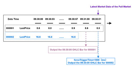
• This example uses DolphinDB’s daily time-series aggregation engine DailyTimeSeriesEngine, which is primarily designed for rolling-window and sliding-window calculations in real-time computing scenarios.
• Setting forceTriggerTime=1000 means that if the latest snapshot time TradeTime for any stock or fund in the entire market is greater than or equal to the window close time (an exact minute boundary in this tutorial) plus 1000 milliseconds (1 second), the system forcibly closes the latest OHLC bar calculation window for inactive stocks and funds and outputs the OHLC bar result. You can set the parameter based on your actual business needs.
• Press enter or click to view image in full size
  
• Setting forceTriggerSessionEndTime=30000 means that once system time reaches each sessionEnd time point, the system waits another 30000 milliseconds (30 seconds) and then forcibly closes the final OHLC bar for any stock or fund that has not yet output its last bar at sessionEnd.

Persist Real-Time OHLC Bars to a Partitioned Table

In the workflow of generating a real-time OHLC bar in this tutorial, there are three stream tables, which contain the following data:

• mdlSnapshotTBName: Raw snapshot data
• mdlSnapshotProcessTBName: Processed raw snapshot data
• mdlStockFundOHLCTBName: 1-minute OHLC bar data

To retain stream table data permanently, we need to persist it in a partitioned table. Using the 1-minute OHLC bar results as an example, the following section explains in detail how to persist newly appended real-time data from a stream table to a partitioned table.

Step 1: Create the Database and Partitioned Table

You only need to run the code that creates the database and partitioned table once. Once the partitioned table is successfully created,​ it remains available. Therefore, you do not need to run it repeatedly.

def createStockFundOHLCDfsTB(dbName, tbName){
 if(existsDatabase(dbUrl=dbName)){
  print(dbName + " has been created !")
  print(tbName + " has been created !")
 }
 else{
  db = database(dbName, VALUE, 2021.01.01..2021.12.31)
  print(dbName + " created successfully.")
  colNames = `SecurityID`TradeTime`OpenPrice`HighPrice`LowPrice`ClosePrice`Volume`Turnover`TradesCount`PreClosePrice`PreCloseIOPV`IOPV`UpLimitPx`DownLimitPx`ChangeRate
  colTypes = [SYMBOL, TIMESTAMP, DOUBLE, DOUBLE, DOUBLE, DOUBLE, LONG, DOUBLE, INT, DOUBLE, DOUBLE, DOUBLE, DOUBLE, DOUBLE, DOUBLE]
  schemaTable = table(1:0, colNames, colTypes)
  db.createPartitionedTable(table=schemaTable, tableName=tbName, partitionColumns=`TradeTime)
  print(tbName + " created successfully.")
 }
 return loadTable(dbName, tbName).schema().colDefs
}
dbName = "dfs://stockFundStreamOHLC"
tbName = "stockFundStreamOHLC"
createStockFundOHLCDfsTB(dbName, tbName)

Step 2: Subscribe to the 1-Minute OHLC Bar Results Table for Real-Time Persistence

Run the following code:

subscribeTable(
 tableName=mdlStockFundOHLCTBName,
 actionName=mdlStockFundOHLCTBName,
 handler=loadTable("dfs://stockFundStreamOHLC", "stockFundStreamOHLC"),
 msgAsTable=true,
 batchSize=5000,
 throttle=1,
 hash=0,
 reconnect=true)

Note:

To improve throughput when writing real-time data to the partitioned table, we recommend setting batchSize to 5000 and throttle to 1 (s) to write data in batches.

Ingest Real-Time Market Data

After you complete the preceding steps, ingest real-time snapshot data into the raw market data table mdlSnapshotTBName to trigger the predefined OHLC bar calculation tasks.

You can ingest real-time market data through DolphinDB market data plugins, message queue plugins, or APIs for various programming languages. For details, refer to the corresponding tutorials.

In this tutorial, historical market data stored in the database is replayed as streaming data by using DolphinDB’s replay feature for debugging and development.

Run the following code to start the replay task:

replayData = select *
  from loadTable("dfs://snapshotDB", "snapshotTB")
  where TradeTime.date()=2023.02.01
  order by TradeTime
replay(
 inputTables=replayData,
 outputTables=mdlSnapshot,
 dateColumn=`TradeTime,
 timeColumn=`TradeTime,
 replayRate=-1)

After the replay finishes, you can run the following code to view the result in the stream table:

result = select * from mdlStockFundOHLC order by SecurityID

You can run the following code to view the result in the partitioned table:

result = select *
 from loadTable("dfs://stockFundStreamOHLC", "stockFundStreamOHLC")
 where SecurityID=`666666

Subscribe from a Python Client

DolphinDB provides subscription APIs for multiple programming languages, including Python, C++, Java, and C#. For details, refer to the corresponding API tutorials.

This tutorial uses Python API as an example to demonstrate a simple third-party client that consumes DolphinDB streaming data. Run the following code in your Python environment:

import dolphindb as ddb

# Establish a session and connection with DolphinDB
s = ddb.session()
s.connect(host="127.0.0.1", port=8848, userid="admin", password="123456")

# Define the callback function in the Python client
def handlerTestPython(msg):
    print(msg)
    
# Enable subscription in the Python client to DolphinDB
s.enableStreaming(0)

# Subscribe
s.subscribe(host="127.0.0.1",
            port=8848,
            handler=handlerTestPython,
            tableName="mdlStockFundOHLC",
            actionName="testStream",
            offset=0,
            batchSize=2,
            throttle=0.1,
            msgAsTable=True)

The output:

Notes:

• In this example, offset is set to 0, which means the subscriber starts consuming from the first historical record stored in memory in the stream table. Therefore, when you start the subscription in Python, the Python client can consume all records in the subscribed stream table.
• In a live market, offset is typically set to -1, which means consumption starts when the subscription starts and processes only the incremental data, namely the latest data appended to the subscribed stream table from that point forward.

Configure the DolphinDB Dashboard

DolphinDB provides a convenient visual dashboard configuration. For detailed instructions, see the official tutorial: Dashboard.

The dashboard configured for the OHLC bar data generated from this tutorial is shown below:

Clean Up the Environment

Real-time computation in this tutorial mainly relies on DolphinDB streaming, including publish-subscribe, stream tables, and the streaming engine. When you clean up the environment, you must clean all of these definitions.

Environment cleanup:

• Before you delete a stream table, you must first remove all related publish-subscribe using the unsubscribeTable.
• Use the dropStreamTable to delete a stream table.
• Use the dropStreamEngine to delete a streaming engine.

You can run the following code to clean up the streaming environment used in this tutorial:

//Declare parameters
mdlSnapshotTBName = "mdlSnapshot"
mdlSnapshotProcessTBName = "mdlSnapshotProcess"
mdlSnapshotProcessEngineName = "mdlSnapshotProcessEngine"
mdlStockFundOHLCTempEngineName = "mdlStockFundOHLCTempEngine"
mdlStockFundOHLCTBName = "mdlStockFundOHLC"
mdlStockFundOHLCEngineName = "mdlStockFundOHLCEngine"
//Cancel related subscriptions
try{unsubscribeTable(tableName=mdlSnapshotTBName, actionName=mdlSnapshotProcessEngineName)} catch(ex){print(ex)}
try{unsubscribeTable(tableName=mdlSnapshotProcessTBName, actionName=mdlStockFundOHLCTempEngineName)} catch(ex){print(ex)}
try{unsubscribeTable(tableName=mdlStockFundOHLCTBName, actionName=mdlStockFundOHLCTBName)} catch(ex){print(ex)}
//Cancel the definition of related stream tables
try{dropStreamTable(mdlSnapshotTBName)} catch(ex){print(ex)}
try{dropStreamTable(mdlSnapshotProcessTBName)} catch(ex){print(ex)}
try{dropStreamTable(mdlStockFundOHLCTBName)} catch(ex){print(ex)}
//Cancel the definition of related stream calculation engines
try{dropStreamEngine(mdlSnapshotProcessEngineName)} catch(ex){print(ex)}
try{dropStreamEngine(mdlStockFundOHLCEngineName)} catch(ex){print(ex)}
try{dropStreamEngine(mdlStockFundOHLCTempEngineName)} catch(ex){print(ex)}

Real-time performance benchmark:

Unified Stream and Batch Processing for Generating OHLC Bars

To support a unified production and research workflow, we need a single codebase to generate OHLC bars from both historical and real-time snapshot data.

To meet this, you only need to follow the tutorial for generating OHLC bars from real-time snapshot data, replay the complete historical dataset at full speed, and then store the resulting OHLC bar output in a partitioned table.

For live real-time computation, simply connect to the real-time market data as described in Section 3.7 of this chapter. If you have any questions, please contact technical support.

Wrapping Up

The transformation from raw snapshot data to clean OHLC bars is deceptively complex. The cumulative nature of high/low prices and volume counters, the uneven snapshot cadence, the special treatment of the opening call auction, and the need to handle illiquid instruments gracefully — each of these requires careful handling.

DolphinDB’s combination of a time-series-native SQL dialect, reactive state engines, and daily time-series engines makes it possible to express this logic concisely and run it at scale: 24 million rows processed in 4.3 seconds historically, sub-millisecond latency in real time.

The rules described here reflect common practice for Chinese equity markets; your own exchange or asset class may have different conventions. But the structural approach — preprocess deltas, aggregate with proper high/low logic, align to a fixed bar grid, forward-fill gaps — translates broadly.

Appendix

• Test data: testData.csv
• Code for generating OHLC bars from historical snapshot data: calHistoryOHLC.dos
• Code for generating OHLC bars from real-time snapshot data: calStreamOHLC.dos