How We Built a Real-Time Implied Volatility Engine for Commodity Options
Every options trader knows the feeling: the market moves, your Greeks shift, and somewhere beneath the noise, there’s a volatility surface trying to tell you something — if only you could read it fast enough.
Press enter or click to view image in full size
Implied volatility (IV) is more than just a number. It’s the market’s collective best guess at future uncertainty, baked into option prices in real time. But raw IV is messy. Tick data is noisy, markets gap, and ever since the 1987 crash exposed the limits of constant-volatility assumptions, traders have known that Black-Scholes is a useful fiction — not a market reality.
In commodity futures markets, the problem compounds: storage costs, seasonal demand, and roll dynamics all distort the standard pricing models. That’s where the Black-76 model comes in — a futures-aware variant of Black-Scholes that strips out the equity assumptions and prices options directly off the futures curve.
In this article, we’ll walk through how to build a real-time IV calculation and volatility smile construction pipeline for commodity options, using DolphinDB’s streaming framework. By the end, you’ll have a working architecture that goes from raw CTP tick data to a smoothed volatility curve — refreshed every minute, live.
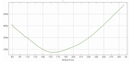
Based on DolphinDB’s streaming processing framework, this tutorial performs real-time calculation of IV and Greeks for commodity options, and fits volatility curves every minute.
1. Overview: What We’re Building and Why
In the futures and options market, real-time IV is typically calculated based on the Black-Scholes (BS) model. The BS model assumes that the underlying price follows a lognormal distribution and derives the theoretical price of a European option from the no-arbitrage pricing principle. Its core formula values an option using five variables: the underlying price, strike price, time to maturity, risk-free interest rate, and volatility. However, the BS model assumes that the underlying asset is infinitely divisible and pays no dividends, which limits its applicability to futures and options. Its variant, the Black-76 model, replaces the underlying price with the futures price and adjusts the pricing logic based on the relationship between the futures and option maturities. This makes it more suitable for commodity futures options and interest rate futures options. In particular, it provides improved accuracy when the underlying involves storage costs or convenience yields. The formulas are as follows:



Where:
- F: current price of the underlying futures contract
- K: option strike price
- T: time to maturity, in years
- r: risk-free interest rate with continuous compounding
- σ: annualized volatility of the futures price
- N(…): cumulative distribution function of the standard normal distribution
This tutorial calculates IV based on the Black-76 model. Common algorithms for calculating IV under the Black-76 model include the Newton-Raphson method, the bisection method, and Brent’s method. Compared with the other two algorithms, Brent’s method combines bisection with inverse quadratic interpolation in a hybrid optimization algorithm that offers both stability and fast convergence. DolphinDB also provides a dedicated function for this method; see brentq for details. For implementations and applications of other algorithms, see the tutorial Calculating ETF Option Implied Volatility and Greeks.
2. System Architecture: How the Pipeline Fits Together
With the Black-76 model and Brent’s method established as our pricing foundation, let’s look at how all the moving parts fit together into a real-time pipeline.
This section explains how DolphinDB uses the streaming engine to implement real-time IV calculation, Greeks calculation, volatility smile construction, and smoothing. The implementation architecture is shown below:
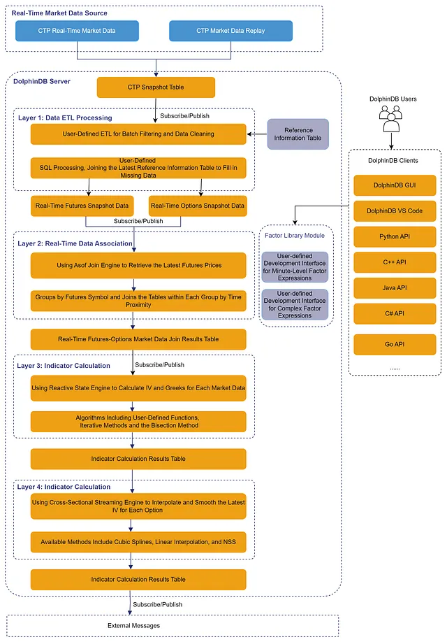
For live trading environments, DolphinDB provides a CTP plugin to ingest tick market data.
For research environments, DolphinDB provides the replay function to replay historical data and simulate real-time market data: Historical Data Replay.
After market data is ingested, the workflow mainly consists of the following steps:
- Data validation and filtering: In this tutorial, real-time market data undergoes a basic filtering process, including conditions such as: bid/ask prices and trading volume must be greater than zero; timestamps must fall within trading hours; and the time difference between data arrival and the actual trade timestamp must not exceed 5 seconds. You can add more filtering rules as needed. During filtering, we also use the reference information table to fill in required fields. After filtering, futures market data and options market data are stored in separate stream tables.
- Futures price selection: To calculate option IV, an appropriate futures price must be determined. In this tutorial, the futures price is selected as the nearest available observation in time relative to each option quote timestamp. This is implemented using DolphinDB’s Asof Join Engine, which performs time-nearest matching between futures and options streams. The resulting dataset combines option prices, the most recent futures prices, and relevant reference information into a single stream table.
- IV and Greeks calculation: As described in previous sections, the model and algorithm methods have already been introduced. Here, a Reactive State Engine is used to calculate IV and Greeks independently for each valid market data record.
- Volatility smile construction and smoothing:
- IV curves are generally constructed from more liquid out-of-the-money (OTM) options. In this example, a real-time volatility curve is constructed every minute. Since some contracts have low trading frequency and may not generate continuous updates, a Cross-Sectional Engine is used instead of a Time-Series Engine. At each timestamp, the latest IV for each strike price is used to construct the curve.
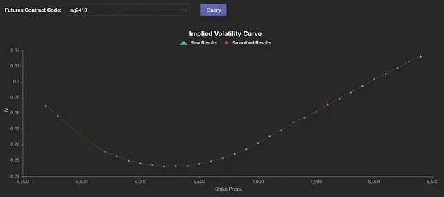
- Curve smoothing: Due to missing observations, market noise, and volatility fluctuations, the resulting volatility curve may appear irregular. To address this, cubic spline interpolation is applied for smoothing. DolphinDB provides a built-in function cubicSpline for this purpose. In addition, functions such as linearInterpolateFit, pchipInterpolateFit, and nss are also available, allowing users to choose the most appropriate method for curve fitting and smoothing according to their needs.
3. The Data: CTP Tick Feeds and Reference Tables
Before diving into the implementation, it’s worth understanding the raw material we’re working with — the CTP tick feeds and reference tables that power every step of this pipeline.
The futures options market data used in this tutorial comes from real-time CTP data. CTP, short for Comprehensive Transaction Platform, is a business management system for the futures market. DolphinDB provides a CTP plugin that connects to the CTP system to subscribe to real-time market data from the futures market and query instrument information. The schema of the CTP real-time market data table is as follows:

In addition to the raw market data, this tutorial also uses futures and options reference data from the CTP system, which is further processed for downstream calculations. The table schema is as follows:

4. Building the Pipeline Step by Step
With the data structure in place, we can now walk through the implementation step by step.
The appendix at the end of this tutorial provides sample data, as well as scripts to create the database and tables, and to import the data. After executing the database and table creation scripts, the following script can be used to import the test data:
YourDir = ""
// Import reference data
schemaInfo = select name,typeString from loadTable("dfs://option_info", "data").schema().colDefs
t = loadText(filename=YourDir+"option_info.csv", schema=schemaInfo)
tableInsert(loadTable("dfs://option_info", "data"), t)
// Import futures and options market data
schemaMarket = select name,typeString from loadTable("dfs://ctp", "market").schema().colDefs
loadTextEx(dbHandle=database("dfs://ctp"), tableName="market", partitionColumns=["TradingDay","InstrumentID"], filename=YourDir+"market.csv", schema=schemaMarket)
Once the import is completed successfully, execute the appendix scripts in the following order: environment_initialization.dos, function_engine_definitions.dos, and data_replay.dos. You can then quickly experience real-time IV calculation and curve construction.
4.1 Futures Price Selection
As mentioned earlier, DolphinDB provides an asof join engine for time-nearest matching between left and right tables. This makes it straightforward to retrieve the nearest futures price based on the option quote timestamp, as shown below:
ajEngine = createAsofJoinEngine(
  name="asofJoin",
  leftTable=ctpOptions,
  rightTable=ctpFutures,
  outputTable=futOptCrt,
  metrics=<[ctpOptions.InstrumentID, ctpFutures.assetCode, (ctpFutures.BidPrice1+ctpFutures.AskPrice1)\2, (ctpOptions.BidPrice1+ctpOptions.AskPrice1)\2, KPrice, CPMode, endDate]>,
  matchingColumn=[[`futureCode],[`InstrumentID]],
  timeColumn=`TradingTime,
  useSystemTime=false)
// subscription topic
subscribeTable(tableName="ctpOptions", actionName="appendLeftStream", handler=getLeftStream(ajEngine), msgAsTable=true, offset=-1, hash=0)
subscribeTable(tableName="ctpFutures", actionName="appendRightStream", handler=getRightStream(ajEngine), msgAsTable=true, offset=-1, hash=1)
Here, option market data is in the left table, and futures market data is in the right table. For each option quote, the engine retrieves the most recent futures quote and outputs the joined result. You can use the delayedTime parameter to configure the timeout-based forced trigger rule. For details, see the Asof Join Engine documentation.
4.2 IV Calculation
The brent function requires a function argument f and finds a root x0 of f(x) over a given interval [a,b] such that f(x0)=0. Therefore, in addition to implementing the Black-76 model, the code also defines a function loss_function that returns the difference between theoretical and market prices, and then solves it with the brent function. The calculation code is as follows:
/** @Brief: Calculates IV using the Black-76 formula
* @Param: F: Current price of the underlying futures contract
* @Param: K: Strike price
* @Param: T: Time to maturity
* @Param: r: Risk-free interest rate
* @Param: sigma: Volatility
* @Param: option_type: Option type, 1 or -1, representing 'C' or 'P'*/
def black_76(F, K, T, r, sigma, option_type){
    d1 = (log(F \ K) + (0.5 * pow(sigma , 2) ) * T) \ (sigma * sqrt(T))
    d2 = d1 - sigma * sqrt(T)
    if (option_type == 1){
        return exp(-r * T) * (F * cdfNormal(0,1,d1) - K * cdfNormal(0,1,d2))
    }else if( option_type == -1){
        return exp(-r * T) * (K * cdfNormal(0,1,-d2) - F * cdfNormal(0,1,-d1))
    }else{
        return ("Option type must be 1 or -1.")
    }
}
/** @Brief: Solver function for IV using Brentq
* @Param: sigma: Volatility
* @Param: F: Current price of the underlying futures contract
* @Param: K: Strike price
* @Param: T: Time to maturity
* @Param: r: Risk-free interest rate
* @Param: option_type: Option type, 1 or -1, representing 'C' or 'P'
* @Param: market_price: Option price*/
def loss_function(sigma, F, K, T, r, option_type, market_price){
    return black_76(F, K, T, r, sigma, option_type) - market_price
}
/*** @Brief: Calculates IV using Brentq
* @Param: F: Current price of the underlying futures contract
* @Param: K: Strike price
* @Param: T: Time to maturity
* @Param: r: Risk-free interest rate
* @Param: option_type: Option type, 1 or -1, representing 'C' or 'P'
* @Param: market_price: Option price
* @Return:
* @Sample usage:*/
def implied_volatility_Black76Brentq(F, K, T, r, option_type, market_price){
 iv = double(NULL)
 try{
   iv = brentq(f=loss_function, a=1e-6, b=2, xtol=2e-12, rtol=1e-9, maxIter=100, funcDataParam=[F, K, T, r, option_type, market_price])[1]
 }catch(ex){
   writeLog("calculate error: " + ex)
 }
 return iv
}
4.3 Volatility Curve Construction and Smoothing
DolphinDB’s cross-sectional engine retains the latest record for each group, effectively addressing missing market data for some contracts due to infrequent trading. In addition, the cross-sectional engine can be triggered at fixed intervals based on event time. Here, a cross-sectional engine is created to construct and smooth volatility curves every minute of event time. The code is as follows:
crossEngine = createCrossSectionalEngine(
  name="crossEngine",
  metrics=<[last(assetCode), buildIVCurve(trigger, futureCode, assetCode, futurePrice, KPrice, CPMode, iv)]>,
  dummyTable=ivResult,
  outputTable=ivCurve,
  keyColumn=`futureCode`KPrice`CPMode,
  triggeringPattern='dataInterval',
  triggeringInterval=60*1000,
  timeColumn=`trigger,
  useSystemTime=false,
  contextByColumn=`futureCode,
  outputElapsedMicroseconds=true)
filterFn = def (msg) { // Filter out records with invalid IV
 return (select * from msg where iv > 0)
}
subscribeTable(tableName="ivResult", actionName="buildCurve", offset=-1, handler=append!{crossEngine}, msgAsTable=true, batchSize=10000, throttle=1, hash=3, filter=filterFn);
In practice, volatility curves are typically constructed using more liquid OTM options. The latest futures price for each minute is used as the benchmark to identify OTM call and put options. The code is as follows:
strikePrices = KPrice[KPrice< lastPrice and CPMode == -1].join(KPrice[KPrice>= lastPrice and CPMode == 1])
strikeIvs = iv[KPrice< lastPrice and CPMode == -1].join(iv[KPrice>= lastPrice and CPMode == 1])
indexes = isort(strikePrices) // Sort
strikePrices = strikePrices[indexes]
strikeIvs = strikeIvs[indexes]
This tutorial applies cubic spline interpolation for curve smoothing. First, a spline model is constructed using the selected OTM options and their implied volatilities. The strike price range is then evenly divided into 50 segments, and the fitted model is used to interpolate implied volatilities at the generated strike prices. Finally, it stores the original strike prices and implied volatilities together with the smoothed strike prices and interpolated implied volatilities in array vectors. The code is as follows:
n = 50 // Sample count
if(strikePrices.size() >= 3 ){ // Do not fit the curve if there are too few volatility data points
 // Construct the strike price coordinates for the smile curve
  curvePrices = linspace(min(strikePrices), max(strikePrices), n, true)[1]$int
 // Construct the cubic spline interpolation model
  cs = cubicSpline(strikePrices, strikeIvs)
  // Interpolate to obtain the volatility data for the smile curve
  curveIvs = cubicSplinePredict(cs, curvePrices)
  // Return the interpolation results
  tableInsert(objByName(`interResult), ( max(trigger), first(futureCode), first(assetCode), arrayVector([strikePrices.size()], strikePrices), arrayVector([strikeIvs.size()], strikeIvs), arrayVector([curvePrices.size()], curvePrices), arrayVector([curveIvs.size()], curveIvs) ))
}else{
  prices, ivs = NULL, NULL
  if(strikePrices.count()>0) prices, ivs = arrayVector([strikePrices.size()], strikePrices), arrayVector([strikeIvs.size()], strikeIvs)
  tableInsert(objByName(`interResult), ( max(trigger), first(futureCode), first(assetCode), prices, ivs, NULL, NULL ))
}
5. Seeing It Live: The Volatility Dashboard
The dashboard brings the full pipeline to life. Let’s step back and look at what we’ve actually built.
DolphinDB provides a visualization Dashboard that enables real-time volatility curve construction with scheduled refresh. The resulting visualization is shown below:
6. Summary
Based on DolphinDB’s streaming processing framework, this tutorial systematically introduces the real-time calculation of IV and Greeks for commodity options, as well as volatility curve construction, fitting and smoothing. It demonstrates how to leverage DolphinDB streaming engines, combined with the Black–76 model and the Brent’s method, to calculate IV and option Greeks in real time. By utilizing mechanisms such as asof joins and cross-sectional engines, the system achieves futures price selection, real-time market data filtering, and dynamic volatility curve construction, followed by cubic spline interpolation for smoothing. Finally, real-time volatility curves are visualized through the DolphinDB Dashboard.
7. Appendices
Database and table creation scripts: database_table_creation.dos
Tutorial dataset: data.zip
Data import script: csv_import.dos
Environment initialization script: 1.environment_initialization.dos
Streaming engine and function definitions: 2.function_engine_definitions.dos
Data replay script: 3.data_replay.dos
Dashboard display template: dashboard.json