Turning Market History into Live Signals: DolphinDB Data Replay Explained

In quantitative trading and real-time analytics, one of the hardest problems is not computing signals — it’s testing them under realistic conditions.
Most backtests run on static historical data, processed in batch mode. But real trading systems are driven by asynchronous, multi-source event streams: orders, trades, and market snapshots arrive at different times, from different feeds, and in strict chronological order. A strategy that works on end-of-day bars may fail catastrophically when exposed to real-time microstructure effects.
To bridge this gap, DolphinDB introduces a powerful concept: data replay — the ability to inject historical data into a streaming engine as if it were happening live.
This article explains how DolphinDB replays historical data into streaming pipelines, and how it enables accurate simulation of real-time trading environments for strategy research, testing, and validation.
What Is Data Replay?
Data replay is the process of feeding static historical data into a stream processing system in chronological order, at a controllable speed, as if the data were being generated in real time.
This allows you to:
- Backtest real-time strategies using real market microstructure
- Validate streaming logic before production deployment
- Reproduce past trading days exactly
- Test latency-sensitive algorithms under realistic conditions
Without native replay support, users would need to manually script record-by-record insertion, which is slow, error-prone, and cannot guarantee correct timing or ordering. DolphinDB solves this at the engine level.
A Quick Example: Replaying Trades for Real-Time OHLC
Let’s start with a simple example: computing 1-minute bars from historical trade data using streaming logic.
First, we define a streaming pipeline exactly as if we were in a live trading system.
// Create input and output stream tables
share(table=streamTable(1:0, `securityID`tradeTime`price`qty,
[SYMBOL,TIMESTAMP,DOUBLE,INT]), sharedName=`trade)
share(table=streamTable(100:0, `tradeTime`securityID`open`high`low`close,
[TIMESTAMP,SYMBOL,DOUBLE,DOUBLE,DOUBLE,DOUBLE]), sharedName=`OHLC)
go
// Create time-series engine
createTimeSeriesEngine(name="timeSeriesDemo", windowSize=60000, step=60000,
metrics=<[first(price),max(price),min(price),last(price)]>, dummyTable=trade,
outputTable=OHLC, timeColumn=`tradeTime, useSystemTime=false, keyColumn=`securityID)
// Subscribe to table trade
subscribeTable(tableName="trade", actionName="OHLCCal", offset=-1,
handler=getStreamEngine("timeSeriesDemo"), msgAsTable=true)
Save mock data in an in-memory table tradeData:
n = 100000
securityID = rand(`000001`000002`600800`300100, n)
tradeTime = concatDateTime(take(2019.11.07 2019.11.08, n),
(09:30:00.000 + rand(int(6.5*60*60*1000), n)).sort!())
price = 10+cumsum(rand(0.02, n)-0.01)
qty = rand(1000, n)
tradeData = table(securityID, tradeTime, price, qty).sortBy!(`tradeTime)
Now we replay this historical table into the live stream:
replay(inputTables=tradeData, outputTables=trade, dateColumn=`tradeTime,
timeColumn=`tradeTime, replayRate=100, absoluteRate=true)
This injects 100 records per second into the stream, triggering OHLC computation exactly as if trades were arriving live.
Replay Modes in DolphinDB
DolphinDB supports three replay modes depending on how many input and output tables are involved.
1-to-1 Replay (Single Stream)
This is the simplest form: one historical table → one stream table.
sqlObj = <select * from loadTable("dfs://trade", "trade") where Date = 2020.12.31>
tradeDS = replayDS(sqlObj=sqlObj, dateColumn=`Date, timeColumn=`Time)
replay(inputTables=tradeDS, outputTables=tradeStream, dateColumn=`Date,
timeColumn=`Time, replayRate=10000, absoluteRate=true)
This script replays data for 2020.12.31 from the trade table of the dfs://trade database into the target table tradeStream at a rate of 10,000 records per second.
This is useful for validating strategies driven by a single feed such as trades or quotes.
However, live trading solution often requires different types of messages working together. For example, financial market data includes multiple types such as tick order, tick trade and snapshots. To better simulate real-time data streams in actual trading, it’s usually necessary to replay these three types of data simultaneously, which introduces the concept of multi-table replay.
N-to-N Replay (Parallel Streams)
When working with multiple data sources (orders, trades, snapshots), DolphinDB can replay them into separate streams:
sqlObj = <select * from loadTable("dfs://order", "order") where Date = 2020.12.31>
orderDS = replayDS(sqlObj=sqlObj, dateColumn=`Date, timeColumn=`Time)
sqlObj = <select * from loadTable("dfs://trade", "trade") where Date = 2020.12.31>
tradeDS = replayDS(sqlObj=sqlObj, dateColumn=`Date, timeColumn=`Time)
sqlObj = <select * from loadTable("dfs://snapshot", "snapshot") where Date =2020.12.31>
snapshotDS = replayDS(sqlObj=sqlObj, dateColumn=`Date, timeColumn=`Time)
replay(inputTables=[orderDS, tradeDS, snapshotDS],
outputTables=[orderStream, tradeStream, snapshotStream],
dateColumn=`Date, timeColumn=`Time, replayRate=10000, absoluteRate=true)
N-to-1 Replay (Heterogeneous)
To preserve true market chronology, DolphinDB introduces heterogeneous replay. Multiple data sources are merged, sorted by event time, and written into a single heterogeneous stream.
For N-to-1 heterogeneous replay, the inputTables parameter of the replay function must be specified as a dictionary referencing multiple data sources, and the outputTables parameter must specify a stream table with a BLOB column for storing binary messages (i.e., a heterogeneous stream table). Here’s an example of heterogeneous multi-table replay:
sqlObj = <select * from loadTable("dfs://order", "order") where Date = 2020.12.31>
orderDS = replayDS(sqlObj=sqlObj, dateColumn=`Date, timeColumn=`Time)
sqlObj = <select * from loadTable("dfs://trade", "trade") where Date = 2020.12.31>
tradeDS = replayDS(sqlObj=sqlObj, dateColumn=`Date, timeColumn=`Time)
sqlObj = <select * from loadTable("dfs://snapshot", "snapshot") where Date =2020.12.31>
snapshotDS = replayDS(sqlObj=sqlObj, dateColumn=`Date, timeColumn=`Time)
inputDict = dict(["order", "trade", "snapshot"], [orderDS, tradeDS, snapshotDS])
replay(inputTables=inputDict, outputTables=messageStream, dateColumn=`Date,
timeColumn=`Time, replayRate=10000, absoluteRate=true)
The output table messageStream has the following schema:
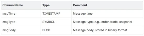
Except for these three required columns, the output table can also contain common columns (with the same name and type) of input tables.
After replay, data of messageStream is shown below:
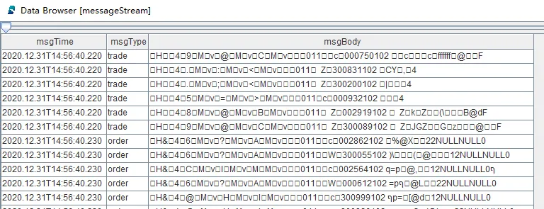
Heterogeneous replay allows global sorting of multiple data sources, ensuring strict chronological order between different data sources. The output heterogeneous stream table can be subscribed like a regular stream table, meaning different types of data can be published by the same table and processed in real-time by the same thread, thus ensuring strict consumption order.
To further process the data of a heterogeneous stream table, such as indicator calculations, the binary-format messages need to be deserialized back to the original format. DolphinDB provides built-in streamFilter for deserializing heterogeneous stream tables and processing the deserialized results. DolphinDB APIs also offer deserializers to extend streaming functionality.
Application Example: Trading Cost Analysis
In data analytics applications, multiple data sources are often required for correlation analysis. For instance, in quantitative strategy development, real-time data processing in production environments is typically event-driven. To accurately simulate real-time streams during live trading in research environments, order, trade, and market snapshots may need concurrent replay for correlated analytics. Heterogeneous multi-table replay is the key to accurately emulating live environments by ensuring absolute chronological order, enabling strategy logic developed and tested during research to fully reproduce actual trading behavior.
The following example demonstrates heterogeneous multi-table replay applied to stock market data.
// Create heterogeneous stream table messageStream
colName = `timestamp`source`msg
colType = [TIMESTAMP,SYMBOL,BLOB]
enableTableShareAndPersistence(table=streamTable(1:0, colName, colType),
tableName="messageStream", asynWrite=true, compress=true, cacheSize=1000000,
retentionMinutes=1440, flushMode=0, preCache=10000)
// Create output table
colName = `TradeTime`SecurityID`Price`TradeQty`BidPX1`OfferPX1`TradeCost`SnapshotTime
colType = [TIME, SYMBOL, DOUBLE, INT, DOUBLE, DOUBLE, DOUBLE, TIME]
enableTableShareAndPersistence(table=streamTable(1:0, colName, colType),
tableName="prevailingQuotes", asynWrite=true, compress=true, cacheSize=1000000,
retentionMinutes=1440, flushMode=0, preCache=10000)
go
// Create join engine
def createSchemaTable(dbName, tableName){
 schema = loadTable(dbName, tableName).schema().colDefs
 return table(1:0, schema.name, schema.typeString)
}
tradeSchema = createSchemaTable("dfs://trade", "trade")
snapshotSchema = createSchemaTable("dfs://snapshot", "snapshot")
joinEngine=createAsofJoinEngine(name="tradeJoinSnapshot", leftTable=tradeSchema,
rightTable=snapshotSchema, outputTable=prevailingQuotes,
metrics=<[Price, TradeQty, BidPX1, OfferPX1, abs(Price-(BidPX1+OfferPX1)/2),
snapshotSchema.Time]>, matchingColumn=`SecurityID, timeColumn=`Time, useSystemTime=false,
delayedTime=1)
// Create stream filter and distribution engine
def filterAndParseStreamFunc(tradeSchema, snapshotSchema){
 filter1 = dict(STRING,ANY)
 filter1["condition"] = "trade"
 filter1["handler"] = getLeftStream(getStreamEngine(`tradeJoinSnapshot))
 filter2 = dict(STRING,ANY)
 filter2["condition"] = "snapshot"
 filter2["handler"] = getRightStream(getStreamEngine(`tradeJoinSnapshot))
 schema = dict(["trade", "snapshot"], [tradeSchema, snapshotSchema])
 engine = streamFilter(name="streamFilter", dummyTable=messageStream,
 filter=[filter1, filter2], msgSchema=schema)
 subscribeTable(tableName="messageStream", actionName="tradeJoinSnapshot",
 offset=-1, handler=engine, msgAsTable=true, reconnect=true)
}
filterAndParseStreamFunc(tradeSchema, snapshotSchema)
// Replay historical data
def replayStockMarketData(){
 timeRS = cutPoints(09:15:00.000..15:00:00.000, 100)
 sqlObj = <select * from loadTable("dfs://trade", "trade") where Date = 2020.12.31>
 tradeDS = replayDS(sqlObj=sqlObj, dateColumn=`Date, timeColumn=`Time,
 timeRepartitionSchema=timeRS)
 sqlObj = <select * from loadTable("dfs://snapshot", "snapshot") where Date =2020.12.31>
 snapshotDS = replayDS(sqlObj=sqlObj, dateColumn=`Date, timeColumn=`Time,
 timeRepartitionSchema=timeRS)
 inputDict = dict(["trade", "snapshot"], [tradeDS, snapshotDS])
 submitJob("replay", "replay for factor calculation", replay,
 inputDict, messageStream, `Date, `Time, 100000, true, 2)
}
replayStockMarketData()
The above script performs full-speed heterogeneous replay of trade and snapshot data by submitting replay as a background job with submitJob. For the output table messageStream, the streamFilter function then deserializes, filters, and distributes the data for real-time correlation and computation of security-level trading costs using an asof join engine.
Conclusion
Data replay is what turns a streaming engine into a true quantitative research platform.
With DolphinDB, you can:
- Reproduce real trading days
- Simulate live environments
- Validate event-driven strategies
- Run historical and real-time logic on the same pipeline
By combining heterogeneous replay, streaming engines, and event-time processing, DolphinDB eliminates the traditional divide between backtesting and live trading.
What you test is what you trade.