10,000 Sensors, 30 Million Records a Day: A Practical Guide to Industrial IoT Data Modeling and Ingestion
Industrial IoT projects often run into the same problem: decisions that seem insignificant early on become expensive later.
When there are only a few devices, choices like schema design, storage engine, and partition strategy rarely matter. But as the number of connected devices and the data volume grow, those early decisions begin to determine whether the system can continue to scale efficiently.
In this article, we'll use a real-world Industrial IoT example to walk through the key decisions behind data modeling in DolphinDB and explore several practical approaches to data ingestion.
A Typical Industrial IoT Scenario
Imagine that in a factory workshop, 10,000 sensors are deployed, reporting temperature, pressure, humidity, voltage, current, and status information every 30 seconds. At this reporting frequency, the system generates nearly 30 million records every day.
For workloads like this, the challenge isn't simply storing the data—it's organizing the data so that it supports continuous high-speed ingestion, efficient queries, and future scalability.
Step 1: Design the Data Model
Before deciding on partitions, there are three questions that should be answered first:
- What fields should be stored?
- Should the data use a wide table or a narrow table?
- Which storage engine best matches the query workload?
1. Schema Design
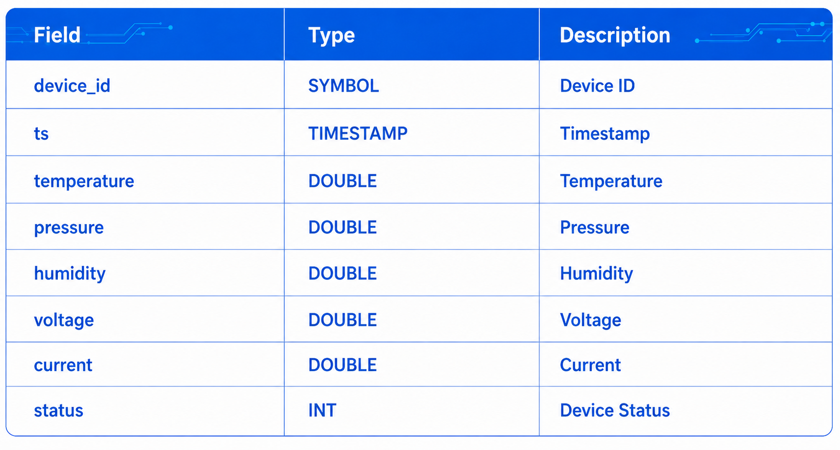
Schema design determines which fields should be stored and which data types should be used. The goal is to capture all sensor information while avoiding unnecessarily large data types that waste storage space.
For this example, the table contains:
2. Wide Table or Long Table?
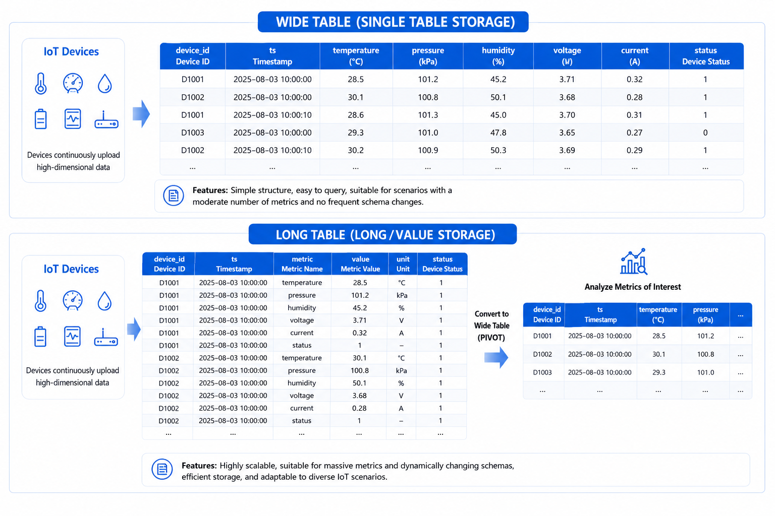
In this scenario, every sensor reports all measurements at exactly the same timestamp, and the set of metrics is relatively stable.
A wide table is therefore the better choice because it:
- simplifies multi-metric queries for a device
- avoids expensive joins
- improves analytical efficiency
If different metrics arrive at different frequencies or new metrics are frequently added, a long table would provide greater flexibility.
3. Choosing the Storage Engine
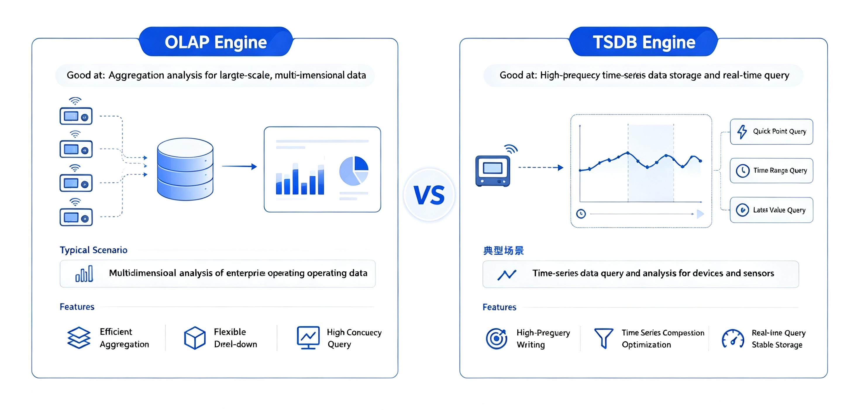
DolphinDB provides two primary storage engines.
The OLAP engine is optimized for large-scale analytical workloads, such as monthly energy consumption statistics across an entire factory.
The TSDB engine is specifically optimized for time-series workloads involving device + time queries. By leveraging partition pruning and sorted indexes, it significantly accelerates point lookups, latest-value queries, and time-range scans.
Since our most common access pattern is retrieving data for a specific device over a period of time, TSDB is the natural choice.
4. Designing the Partition Strategy
Partitioning is one of the most important mechanisms for organizing large datasets in DolphinDB.
When query conditions include partition keys, only the relevant partitions need to be scanned, dramatically reducing disk I/O. On the other hand, partitions that are too large or too small can both hurt performance.
Partition design should be based on two factors:
- The most common query conditions. In this case, queries are primarily filtered by device ID and timestamp, making them ideal partition candidates.
- Recommended partition size for the storage engine. Each storage engine has practical guidelines for partition granularity.
Estimate the Data Volume
Estimate the data volume based on the schema:
- Row size ≈ 4 bytes (device_id) + 8 bytes (ts) + 8 × 5 bytes (five DOUBLE metrics) + 4 bytes (status) = 56 bytes
- Daily data volume ≈ 28,800,000 rows × 56 bytes ≈ 1.5 GB
AFor TSDB, the recommended partition size is 400 MB–1 GB, so date-only partitioning would create oversized partitions (~1.5 GB/day).
A better choice is VALUE partitioning by date + HASH partitioning by device ID, with 4–5 HASH partitions planned upfront, as the partition count is difficult to change after database creation.
Step 2: Create the Database and Table
// Step 1: Create a composite partitioned database
create database "dfs://iot_sensor"
partitioned by VALUE(2025.01.01..2025.01.03), HASH([SYMBOL, 5])
engine="TSDB"

// Step 2: Create the partitioned table
create table "dfs://iot_sensor"."sensor_data"(
    device_id SYMBOL[comment="Device ID"],
    ts TIMESTAMP[comment="Timestamp", compress="delta"],
    temperature DOUBLE,
    pressure DOUBLE,
    humidity DOUBLE,
    voltage DOUBLE,
    current DOUBLE,
    status INT
)
partitioned by ts, device_id
sortColumns=["device_id","ts"]
Three configuration choices are particularly important here.
1. Use the TSDB Engine
TSDB is designed for high-frequency time-series workloads, especially queries filtered by device and time, as well as window aggregations.
2. Partition by Both Timestamp and Device ID
The table definition directly reflects the composite partition strategy discussed earlier.
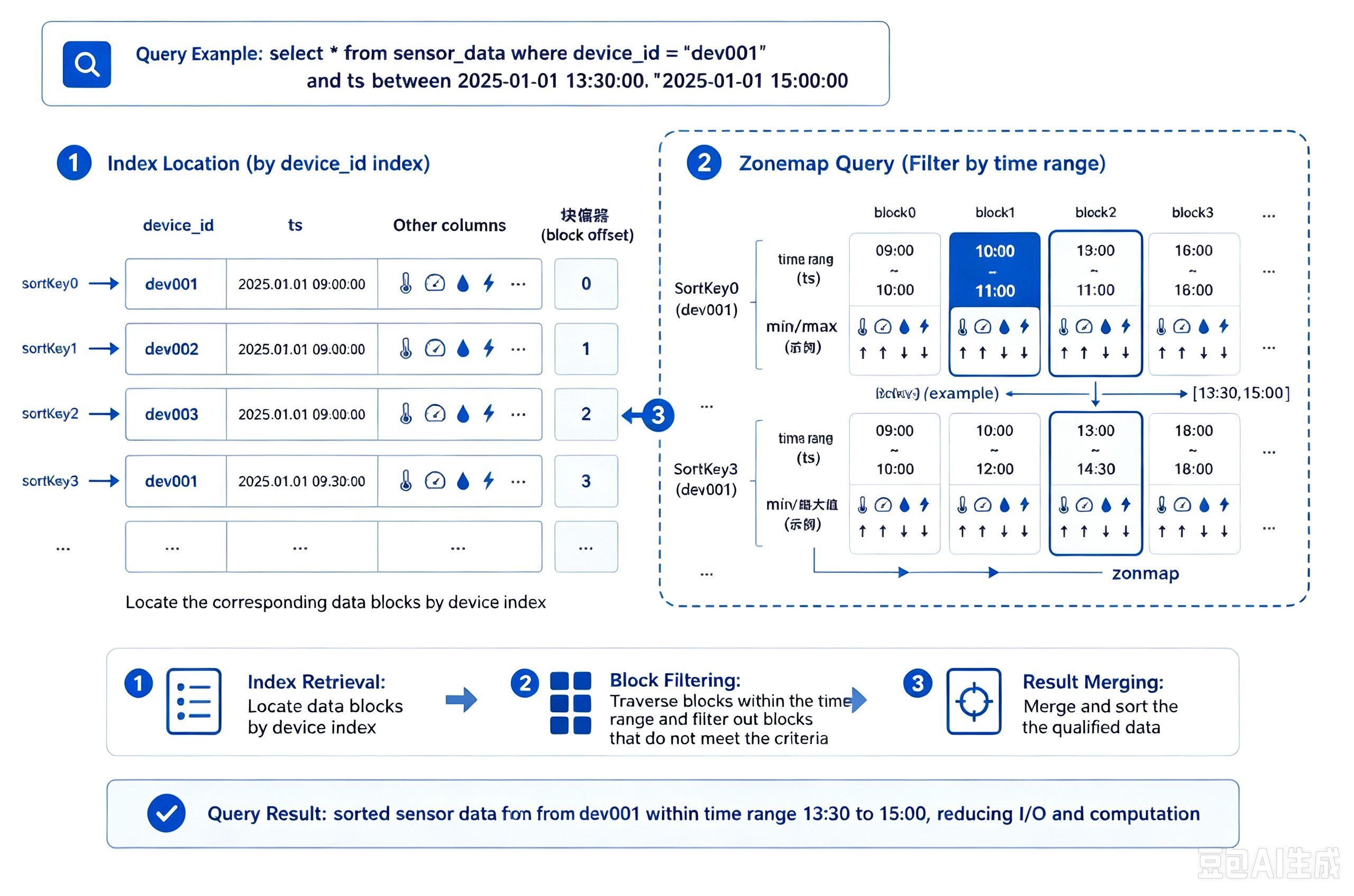
3. Sort by device_id and ts
Sort columns determine how data is physically organized inside each partition.
The last sort column must be the time column. By sorting first on device_id and then on ts, queries for a particular device can efficiently leverage TSDB's internal indexes.
Step 3: Ingest the Data
Industrial IoT systems rarely have a single data source. The appropriate ingestion method depends on how data enters the system.
Option 1. Batch Writes Through APIs
This approach is well suited for gateways or edge services that upload data periodically in batches.
DolphinDB provides client APIs for Python, Java, Go, and C++, making it easy to integrate applications with the database.
A simple Python example:
import dolphindb as ddb
import pandas as pd

# Connect
s = ddb.session()
s.connect("127.0.0.1", 8848, "admin", "123456")

# Prepare data
data = pd.DataFrame({...})

# Upload to session
s.upload({"data": data})

# Write into the distributed table
s.run("""
pt = loadTable("dfs://iot_sensor", "sensor_data")
tableInsert(pt, data)
""")

print("Write successful")
Depending on data volume and latency requirements, the DolphinDB API offers several write methods.
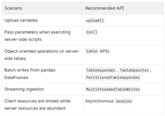
As a general guideline:
- For small or medium batch workloads, tableInsert() or TableAppender is sufficient.
- For high-throughput real-time ingestion, MultithreadedTableWriter or PartitionedTableAppender is recommended because data is automatically routed to the appropriate partitions.
Note: Due to Python's Global Interpreter Lock (GIL), multi-threaded PartitionedTableAppender does not always outperform the single-threaded TableAppender. Benchmarking with your actual workload is recommended.
Option 2. Subscribe to Message Queues
For real-time pipelines built around Kafka, MQTT, or similar middleware, message queues decouple devices from downstream analytics while smoothing traffic spikes.
DolphinDB provides plugins for Kafka, MQTT, RabbitMQ, RocketMQ, and many other messaging systems.
Kafka integration requires only a few lines of code:
loadPlugin("kafka")

consumer = kafka::consumer(...)
kafka::subscribe(...)
kafka::createSubJob(...)
Option 3. Migrate Historical Data
When migrating historical data from systems such as MySQL or Oracle, DolphinDB provides multiple integration options.
These include:
- Dedicated plugins for MySQL, MongoDB, Redis, HBase, and more
- A generic ODBC plugin for databases that provide ODBC drivers
- A dolphindbwriter plugin built on DataX for offline synchronization from a wide range of data sources
The following example imports historical data through ODBC:
loadPlugin("odbc")
conn = odbc::connect("DSN=OracleDB;UID=iot_user;PWD=iot_password")
t = odbc::query(conn, "select device_id, ts, temperature, pressure, humidity, voltage, current, status from sensor_history")
pt = loadTable("dfs://iot_sensor", "sensor_data")
tableInsert(pt, t)
Option 4. Import Files
For CSV or TXT files, DolphinDB provides built-in functions such as loadText() and loadTextEx().
For specialized file formats, dedicated plugins are also available:
- Parquet for efficient columnar storage
- Apache Arrow for cross-platform data exchange and automatic type conversion
- HDF5 for high-frequency scientific and laboratory data
- ZIP for compressed archives
A simple CSV import looks like this:
// Load a small CSV into memory
data = loadText("/path/to/small_data.csv")

// Clean the data
cleanData = select *
from data
where time between 09:00:00 and 16:00:00

// Append to the distributed table
pt = loadTable("dfs://iot_sensor", "sensor_data")
tableInsert(pt, cleanData)
loadText() loads data into an in-memory table, making it easy to inspect fields, preview records, and clean data before writing it to persistent storage.
Final Thoughts
Successful Industrial IoT data platforms are built long before the first line of ingestion code is written.
The key questions are straightforward:
- Where does the data come from?
- How much data will the system generate?
- What are the most common query patterns?
Compared with traditional relational databases, DolphinDB is designed to handle high-frequency ingestion, time-series queries, and large-scale analytics within a unified platform. Storage, computation, and data ingestion are tightly integrated, reducing both system complexity and future development effort.
For workloads centered around device + time, combining the TSDB engine, VALUE partitions on date, HASH partitions on device ID, and a wide-table schema provides an architecture that balances ingestion performance, query efficiency, and long-term scalability.
On the ingestion side, DolphinDB offers a complete toolkit as well:
- APIs and file imports for batch ingestion
- Kafka, MQTT, and other messaging systems for real-time streaming
- Database connectors and migration plugins for historical data import
Getting the data model and ingestion strategy right from the beginning makes it much easier to scale from thousands of devices to tens of thousands—without having to redesign the entire system later.