In a typical industrial IoT environment, 10,000 sensors can generate nearly 30 million records every day. We've previously covered how to design the database and store this volume of time-series data in DolphinDB. But storing all that data is only half the challenge. Once the data is in place, the next question is straightforward: How do we turn millions of raw records into metrics that operators can actually use?

Which machines have the highest or lowest OEE? Which ones are frequently starting and stopping? Which machines are operating abnormally? And how healthy is a production line today?

This article focuses on a common industrial IoT workload: offline batch processing. Using the 10,000-sensor scenario, we'll explore how DolphinDB can turn massive time-series data into actionable metrics for equipment monitoring, anomaly detection, idle-state identification, and operational analysis.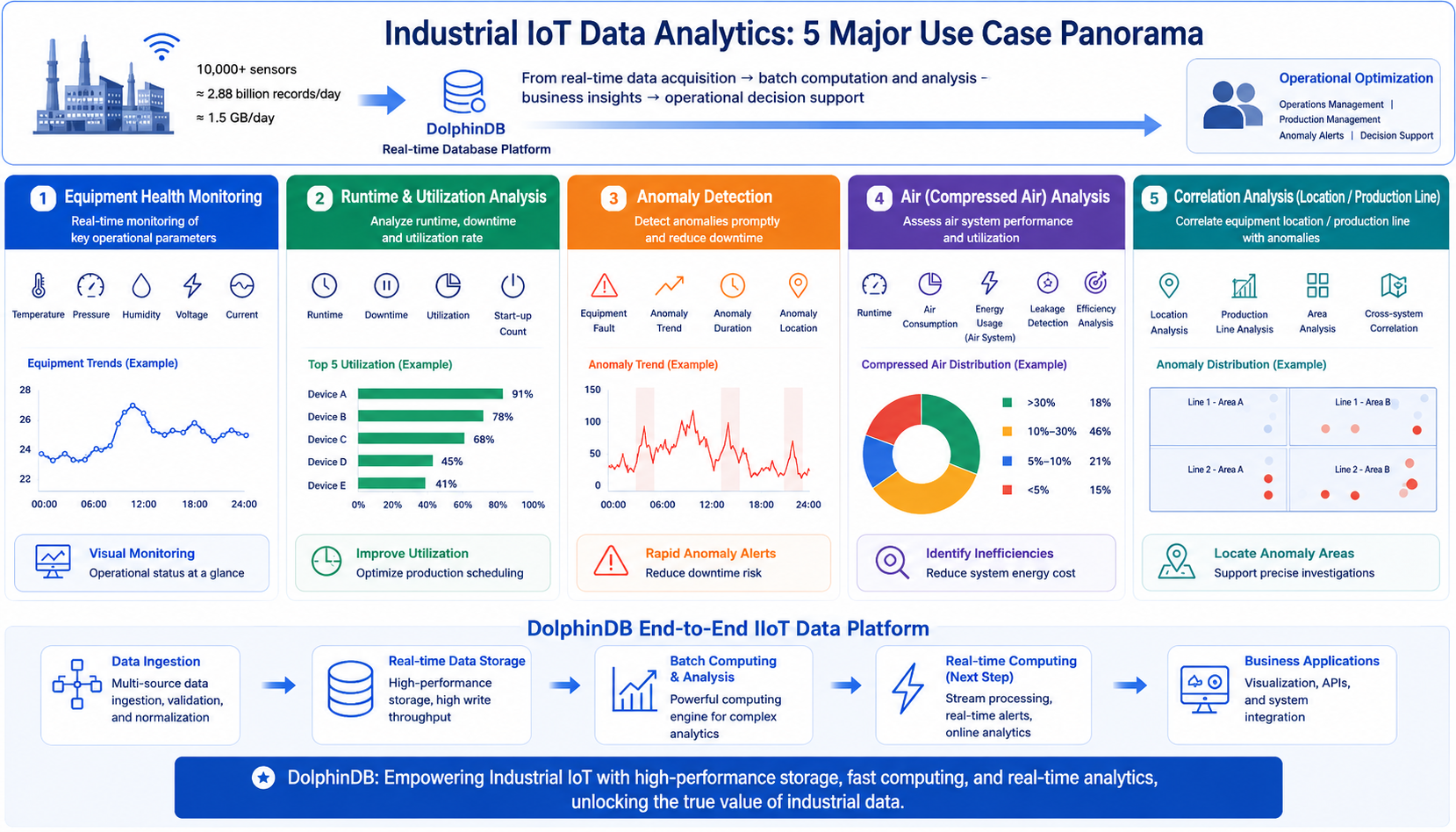

10,000 Sensors, 30 Million Records

We use the same industrial IoT scenario: 10,000 sensors generating nearly 30 million records per day. Each sensor reports temperature, pressure, humidity, voltage, current, and equipment status every 30 seconds. The data can be stored and processed using the DolphinDB Community Edition.

With the data now in place, the next question is: How do we turn tens of millions of raw records into useful business metrics?

We’ll use DolphinDB to tackle several common industrial IoT batch-processing tasks:

Generate equipment operation reports
Calculate operating/downtime and startup/shutdown counts
Detect abnormal equipment states
Identify idle or lightly loaded equipment
Analyze anomalies by location, production line, and other attributes

Scenario 1: Generate an Equipment Operation Report

A common question in industrial operations is: How did the equipment perform yesterday? Querying 30 million raw records directly would return too much detail to be useful.

A better approach is to downsample the high-frequency data into time windows. For example, if data arrives every 30 seconds, we can aggregate it into 10-minute windows:

select
    device_id,
    ts_bar,
    avg(temperature) as temp_avg,
    max(humidity) as humidity_max
from
    loadTable("dfs://iot_sensor", "sensor_data")
where
    ts between 2025.01.01T00:00:00.000
    and 2025.01.01T00:59:59.999
group by
    device_id,
    bar(ts, 10m) as ts_bar

For time-based grouping, DolphinDB provides the bar function, which aligns timestamps to fixed intervals for efficient downsampling.

bar(ts, 10m) groups data into 10-minute buckets, reducing 2,880 daily samples per device to just 144 points for trend reports.

What If Data Is Missing?

In practice, devices may miss reports due to network issues or equipment failures.

The interval function can fill these gaps with nulls or linear interpolation, keeping the time series complete for trend analysis and anomaly detection.

select device_id,
       ts,
       avg(temperature) as temp_avg,
       max(humidity) as humidity_max
from 
      loadTable("dfs://iot_sensor", "sensor_data")
where 
      date(ts) = 2025.01.01
group by 
      device_id, 
      interval(ts, 1m, "prev") as ts

Scenario 2: How Long Was the Equipment Actually Running?

Average temperature and maximum pressure are only basic metrics. A more important question is: How long was the equipment actually running? Operating and downtime are key metrics for lifecycle management and OEE.

Suppose status = 1 means running and status = 0 means stopped. We can use bar(ts, 10m) to group data into 10-minute windows, then calculate cumulative operating and downtime by status:

select
    device_id,
    status,
    ts,
    sum(duration_ms) / 60000.0 as duration_minutes
from
    (
        select
            device_id,
            ts,
            status,
            iif(isNull(next(ts)), 0, next(ts) - ts) as duration_ms
        from
            loadTable("dfs://iot_sensor", "sensor_data")
        where
            device_id = "device_0001"
        and 
            date(ts) = 2025.01.01 
        context by 
            device_id 
        csort 
            ts
    )
group by
    device_id,
    status,
    bar(ts, 10m) as ts

The result is no longer a collection of raw sensor records, but a set of business-ready metrics:

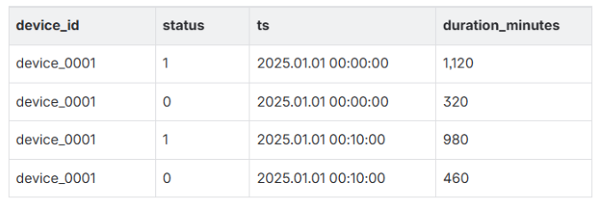
This gives operations teams daily operating and downtime, run/stop ratios, and OEE availability.

We can also count startup and shutdown events. Frequent switching between running and stopped states may indicate abnormal conditions or an imbalanced production cycle.

In DolphinDB, the deltas function calculates changes between consecutive status values: 1 means startup and -1 means shutdown. Counting these transitions gives the total number of startups and shutdowns.

select
    device_id,
    sum(iif(deltas(status) == 1, 1, 0)) as start_count,
    sum(iif(deltas(status) == -1, 1, 0)) as stop_count
from
    loadTable("dfs://iot_sensor", "sensor_data")
where
    device_id = 'device_0001'
and 
    date(ts) = 2025.01.01
group by
    bar(ts, 10m),
    device_id

Scenario 3: Detecting Abnormal States

Another common industrial analytics task is anomaly detection: find every threshold violation that occurred yesterday. For example, if the normal temperature range is 20–80°C, we can directly filter the historical data for readings outside that range:

select
    device_id,
    ts,
    temperature
from
    loadTable("dfs://iot_sensor", "sensor_data")
where
    date(ts) = 2025.01.01
    and (
        temperature > 80
        or temperature < 20
    )

This answers a straightforward question: Which devices experienced abnormal temperatures yesterday?

If we also need to detect sudden changes, we can calculate the rate of change between consecutive readings:

select
    *
from
    (
        select
            ts,
            device_id,
            current,
            percentChange(current) as changePct
        from
            loadTable("dfs://iot_sensor", "sensor_data")
        where
            device_id = 'device_0001'
            and date(ts) = 2025.01.01
    ) t
where
    abs(t.changePct) > 1

The percentChange function calculates the percentage change between consecutive values, making it easy to detect sudden sensor shifts. Here, we flag changes greater than 100%.

This moves anomaly detection beyond “Did the value exceed the threshold?” to “Did the value change unexpectedly?”

DolphinDB provides many similar built-in functions for time-series calculations, making common analysis tasks more concise and reducing custom logic.

Scenario 4: Detecting Idle Equipment

A subtler form of inefficiency than downtime is when equipment is running but current remains low, indicating it may be idle or lightly loaded.

For example, if current below 20 indicates low load, we can calculate the time spent in this state:

select
    device_id,
    sum(deltas(ts)) / 60000 as no_load_minutes
from
    loadTable("dfs://iot_sensor", "sensor_data")
where
    device_id = 'device_0001'
    and current < 20
    and date(ts) = 2025.01.01
group by
    bar(ts, 10m),
    device_id

Combined with operating time, this helps identify machines with high idle ratios and production lines with excessive unproductive runtime, revealing potential causes of low equipment utilization.

That’s the real value of offline batch processing: turning raw sensor data into actionable metrics for equipment and production management.

Scenario 5: Where Did the Anomaly Occur?

Finding an abnormal temperature on device_0001 is only the first step. We also need to know: Where is the device? What type is it? Which production line does it belong to?

This requires combining OT sensor data with IT-side equipment metadata, such as device name, location, and model. Suppose this information is stored in a separate device_metadata table:

// Create equipment metadata table (in-memory example)
device_list = "device_" + string(1..10000).lpad(4, "0")
device_metadata = table(
    device_list as id,
    take(["Factory_A", "Factory_B", "Factory_C"], 10000) as location,
    take(["Type_A", "Type_B"], 10000) as device_type
) 
// Join to retrieve data for devices located in Factory_A
select
    d.location,
    s.device_id,
    s.temperature,
    s.ts
from
    loadTable("dfs://iot_sensor", "sensor_data") s
    inner join device_metadata d on s.device_id = d.id
where
    d.location = 'Factory_A'
    and date(s.ts) = 2025.01.01

This enables location-based anomaly tracing: Which devices in Factory_A had anomalies, when did they occur, and what were the readings?

This matters because industrial analytics ultimately needs to connect database records to real-world equipment, production lines, and manufacturing processes.

DolphinDB supports standard SQL joins as well as time-series joins such as as-of join and window join, which are useful when timestamps don't align:

As-of join: Matches each sensor reading with the most recent historical record, such as equipment status or maintenance data.
Window join: Links data within a specified time window, such as calculating temperature or pressure around an alarm event.

Summary

We have focused on how to store nearly 30 million records generated by 10,000 sensors every day. This chapter moved to the next question: How do we turn that data into real value?

We covered common batch-processing tasks including equipment monitoring, anomaly detection, idle-state identification, and metadata analysis, taking industrial IoT data from storage to practical analytics.

DolphinDB provides an integrated workflow from data ingestion and time-series storage to batch and real-time analytics, making massive sensor data easier to process and put to work.

Next, we'll move from batch processing to real-time stream processing, covering second-level alerts, real-time OEE, online inference, and edge-device integration.

5 Operational Metrics You Can Build From Raw IIoT Data