Building a Real-Time Stock Momentum Ranking System with DolphinDB Stream Processing
Imagine you're running a quant desk. 5,000 stocks are ticking in real time. Every new trade arrives, and your system needs to — instantly — answer two questions:
- How much has each stock moved compared to where it was two minutes ago?
- Across the whole market, which stocks are leading and which are lagging?
In a traditional database, question one alone is already painful: you'd need to store historical snapshots, join them against incoming data, and compute the percentage change — for every single symbol, on every single tick. Question two makes it worse, because you now need to wait until all stocks have been updated before you can rank them meaningfully.
This is the core challenge of real-time factor computation. The calculations are simple in theory, but keeping them stateful, low-latency, and correct across thousands of symbols simultaneously is a different problem entirely.
DolphinDB's streaming framework is built for exactly this. In this post, we'll walk through how to compute real-time Price Rate of Change (ROC) and derive a live market ranking from it — using two composable streaming engines chained into a single pipeline.
What Is ROC and Why Is It Hard in Real Time?
Price Rate of Change (ROC) measures the percentage gain or loss of a stock relative to a past price:
ROC = (current price / price N periods ago) - 1The difficulty is in "N periods ago." In a static dataset, you'd use a window function. But in a live stream, you need to:
- Remember history for each symbol independently
- Handle event time, not machine time — if data arrives late or out of order, the "2 minutes ago" reference should still be based on the event timestamp, not when the message was processed
- Update incrementally — recomputing the full window on every tick doesn't scale
DolphinDB's Reactive State Engine handles all of this. It maintains per-symbol state across events, and many of its built-in functions (like tmove, prev, ratios, cumfirstNot) are incrementally optimized — meaning they update in O(1) rather than reprocessing the entire window each time.
Step 1 — Stateful ROC with the Reactive State Engine
Defining the Factor
DolphinDB uses a @state decorator to mark functions that maintain state across events. Here's a ROC function using tmove, which retrieves the value from a time-based moving window anchored to event time:
@state
def priceChange(datetime, lastPrice, duration){
    return lastPrice \ tmove(datetime, lastPrice, duration) - 1
}
tmove(datetime, lastPrice, 2m) returns the last price recorded at least 2 minutes before the current event's timestamp.
Setting Up the Engine
// Input stream: raw tick data
share(table=streamTable(1:0, `securityID`datetime`lastPrice`openPrice,
    [SYMBOL, TIMESTAMP, DOUBLE, DOUBLE]), sharedName=`tick)

// Output stream: computed factors
share(table=streamTable(10000:0, `securityID`datetime`factor,
    [SYMBOL, TIMESTAMP, DOUBLE]), sharedName=`resultTable)

go

// Create the reactive state engine
createReactiveStateEngine(
    name="reactiveDemo",
    metrics=<[datetime, priceChange(datetime, lastPrice, 2m)]>,
    dummyTable=tick,
    outputTable=resultTable,
    keyColumn="securityID"
)

// Subscribe to tick data
subscribeTable(tableName="tick", actionName="reactiveDemo",
    handler=getStreamEngine(`reactiveDemo), msgAsTable=true, offset=-1)
The keyColumn="securityID" is key here — the engine partitions its internal state by symbol. Each stock gets its own independent state machine.
Choosing the Right ROC Formula
Not all ROC calculations look the same. Here's a practical guide to the four most common patterns and when to use each:
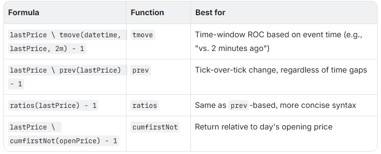
All four functions are incrementally optimized inside the Reactive State Engine. The engine won't reprocess a window from scratch — it updates the rolling state with each new data point.
Step 2 — Cross-Sectional Ranking
Once we have per-symbol ROC values flowing into resultTable, the next step is ranking them across the market. This is a fundamentally different kind of computation: instead of looking at one symbol's history, we're looking at all symbols at the same point in time.
DolphinDB's Cross-Sectional Engine is designed for exactly this. It collects the latest value for each key (symbol), and when triggered, computes a metric across all of them simultaneously.
// Output table for rankings
share(table=streamTable(1:0, `datetime`securityID`factor`rank,
    [TIMESTAMP, SYMBOL, DOUBLE, LONG]), sharedName=`rankTable)

go

createCrossSectionalEngine(
    name="crossSectionalEngine",
    metrics=<[securityID, factor, rank(factor, ascending=false)+1]>,
    dummyTable=resultTable,
    outputTable=rankTable,
    keyColumn=`securityID,
    triggeringPattern='perBatch',
    useSystemTime=false,
    timeColumn=`datetime
)

subscribeTable(tableName="resultTable", actionName="crossSectionalDemo",
    handler=getStreamEngine(`crossSectionalEngine), msgAsTable=true, offset=-1)
A few things worth noting:
- triggeringPattern='perBatch' means a ranking is computed every time a new batch of data arrives.
- useSystemTime=false with timeColumn=`datetime ensures the engine uses event timestamps to determine the "latest" value per symbol
- rank(factor, ascending=false)+1 produces a 1-based descending rank (rank 1 = highest ROC)
Step 3 — Chaining Them into a Pipeline
So far, we have two separate subscriptions: tick → ROC, then ROC results → ranking. Each hop involves writing to a stream table, triggering pub/sub overhead, and potentially switching threads.
DolphinDB lets us eliminate the intermediate stream table entirely by directly wiring one engine's output into another's input:
// Tables
share(table=streamTable(1:0, `securityID`datetime`lastPrice,
    [SYMBOL, TIMESTAMP, DOUBLE]), sharedName=`tick)
share(table=streamTable(10000:0, `securityID`datetime`factor,
    [SYMBOL, TIMESTAMP, DOUBLE]), sharedName=`resultTable)
share(table=streamTable(1:0, `datetime`securityID`factor`rank,
    [TIMESTAMP, SYMBOL, DOUBLE, LONG]), sharedName=`rankTable)

go

// Build the cross-sectional engine first (it's downstream)
createCrossSectionalEngine(
    name="crossSectionalEngine",
    metrics=<[securityID, factor, rank(factor, ascending=false)+1]>,
    dummyTable=resultTable,
    outputTable=rankTable,
    keyColumn=`securityID,
    triggeringPattern='perBatch',
    useSystemTime=false,
    timeColumn=`datetime
)

// Build the reactive state engine, pointing its output at the cross-sectional engine
@state
def priceChange(datetime, lastPrice, duration){
    return lastPrice \ tmove(datetime, lastPrice, duration) - 1
}

createReactiveStateEngine(
    name="reactiveDemo",
    metrics=<[datetime, priceChange(datetime, lastPrice, 2m)]>,
    dummyTable=tick,
    outputTable=getStreamEngine(`crossSectionalEngine),  // <-- pipeline wiring
    keyColumn="securityID"
)

// Only one subscription needed
subscribeTable(tableName="tick", actionName="reactiveDemo",
    handler=getStreamEngine(`reactiveDemo), msgAsTable=true, offset=-1)
The key line is outputTable=getStreamEngine(`crossSectionalEngine). Instead of writing to resultTable and waiting for a subscriber to pick it up, the ROC engine pushes its output directly into the ranking engine's input queue.
Note that resultTable in this setup is only used as a schema template (so the cross-sectional engine knows what columns to expect). It will never actually receive data.
What Else Can You Build With This Pattern?
The two-engine pipeline — stateful time-series computation feeding a cross-sectional aggregation — is a general pattern that maps to a lot of real-world use cases:
- Volatility ranking: replace ROC with a rolling standard deviation of returns, then rank across the market
- Relative volume screening: compute each stock's volume ratio (current vs. 30-day average), then filter for unusual spikes
- Risk alerts: track rolling drawdown per position, then trigger an alert when any position breaches a threshold
- Factor construction: combine multiple per-symbol metrics (momentum, mean reversion, volatility) into a composite score, then rank for portfolio construction
The same structural pattern applies: a reactive state engine handles per-symbol stateful history, and a cross-sectional engine handles the market-wide view.
Wrapping Up
Real-time factor computation is one of those problems that looks simple on paper but has a lot of hidden complexity: state management per symbol, event-time semantics, and the challenge of correctly computing cross-sectional metrics without latency. DolphinDB's streaming engines — and particularly the ability to wire them together into a pipeline — offer a clean solution to all three.
The approach scales naturally: adding new factors means adding new @state functions, and adding new cross-sectional views means adding more downstream engines. The architecture stays the same.
If you want to explore further, DolphinDB's documentation covers additional engine types (anomaly detection, session window, time-series joins) that compose using the same pipeline model.
Thanks for reading. If you found this useful, consider following for more posts on real-time data infrastructure and quantitative systems.