Stop Waiting for Insights: Building Streaming Analytics with DolphinDB
Real-time data processing lies at the heart of modern trading systems, IoT platforms, and operational intelligence pipelines. DolphinDB addresses these needs through its Streaming Engines—encapsulated computation units designed for low-latency analytics over continuous data flows.
In this post, we explore DolphinDB’s streaming engine architecture and walk through practical examples, including:
- Window aggregation for capital flow analysis
- Stateful calculations such as price rate of change (ROC)
- Cross-sectional rankings
- Streaming pipelines
- Real-time joins
- Complex event processing for trading strategies
What Are Streaming Engines?
Streaming engines are independent computing components that subscribe to stream tables, perform real-time calculations, and publish results to downstream tables or engines.
DolphinDB provides more than a dozen built-in engines, enabling flexible real-time processing patterns across financial markets, energy systems, and IoT workloads.
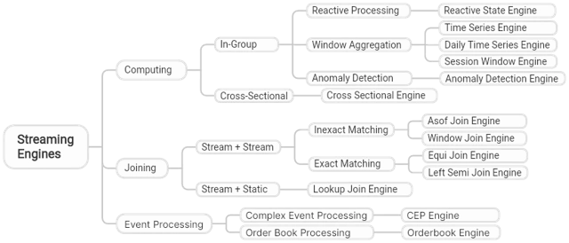
Computing engines are further divided into in-group and cross-sectional computation:
- In-group time series computing: Data is grouped and processed in one of three ways:Row-by-row computationAggregation over windowsAnomaly detection within each group
- Cross-sectional computing: Selects the latest record per group for cross-sectional computation.
Joining engines, similar to SQL JOIN operations, are designed for real-time correlation between two tables. The left table is always a stream table, while the right table can be either a stream or static table:
- Stream + stream join: Values are matched exactly or inexactly based on time series relationships.
- Stream + static join: The stream table is dynamically joined with a snapshot of the right table, which can be either a stream or static table.
Complex event processing engines are tailored for advanced processing over complex events:
- Order Book Engine: Maintains and updates order book with predefined rules from trade and order data.
- CEP Engine: Monitors events from multiple sources and processes events with specified patterns to extract information.
The following sections demonstrate these streaming features with use cases.
Window Aggregation: 1-Minute Capital Flow
Given stock trade data with fields like tradeTime, securityID, price, and qty, we define the following metrics for measuring capital flow:
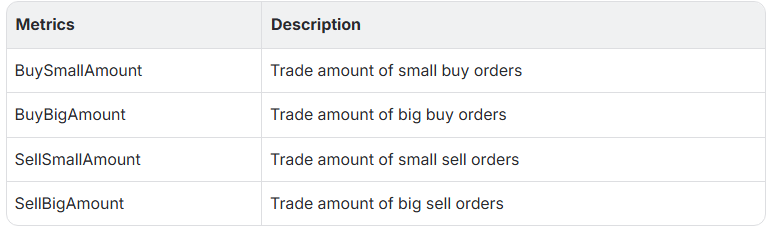
A trade is classified as small if quantity ≤ 50,000 and big otherwise.
These factors can be expressed as follows in DolphinDB:
defg calCapitalFlow(buyNo, sellNo, qty, price){
	smallBigBoundary = 50000
	tempTable1 = select buyNo, sellNo, qty, price,
		iif(buyNo>sellNo, `B, `S) as BSFlag, iif(buyNo>sellNo, `B, `S) as orderNo
		from table(buyNo as `buyNo, sellNo as `sellNo, qty as `qty, price as `price)
	tempTable2 = select sum(qty) as qty, sum(qty*price) as tradeAmount
		from tempTable1 group by orderNo, BSFlag
	buySmallAmount = exec sum(tradeAmount)
		from tempTable2 where qty<=smallBigBoundary && BSFlag==`B
	buyBigAmount = exec sum(tradeAmount)
		from tempTable2 where qty>smallBigBoundary && BSFlag==`B
	sellSmallAmount = exec sum(tradeAmount)
		from tempTable2 where qty<=smallBigBoundary && BSFlag==`S
	sellBigAmount = exec sum(tradeAmount)
		from tempTable2 where qty>smallBigBoundary && BSFlag==`S
	return nullFill([buySmallAmount, buyBigAmount, sellSmallAmount, sellBigAmount], 0)
}
This function becomes the metric inside a time-series engine with rolling or sliding windows:
// Create input and output stream tables
share(table=streamTable(1:0, `tradeTime`securityID`price`qty`buyNo`sellNo,
[TIMESTAMP, SYMBOL, DOUBLE, LONG, LONG, LONG]), sharedName=`trade)
share(table=streamTable(1:0,
`tradeTime`securityID`buySmallAmount`buyBigAmount`sellSmallAmount`sellBigAmount,
[TIMESTAMP,SYMBOL,DOUBLE,DOUBLE,DOUBLE,DOUBLE]), sharedName=`capitalFlow)
go
// Create time-series engine
createTimeSeriesEngine(name="tradeTSAggr", windowSize=60000, step=60000,
metrics=[<calCapitalFlow(buyNo, sellNo, qty, price)>], dummyTable=trade,
outputTable=capitalFlow, timeColumn="tradeTime", useSystemTime=false, keyColumn=`securityID)
// Subscribe to table trade
subscribeTable(tableName="trade", actionName="tradeTSAggr", offset=-1,
handler=getStreamEngine("tradeTSAggr"), msgAsTable=true)
Modify the engine definition for calculation with sliding windows based on tradeTime:
createTimeSeriesEngine(name="tradeTSAggr", windowSize=60000, step=30000,
metrics=[<calCapitalFlow(buyNo, sellNo, qty, price)>], dummyTable=trade,
outputTable=capitalFlow, timeColumn="tradeTime", useSystemTime=false, keyColumn=`securityID)
Modify the engine definition for calculation with sliding windows based on system time:
createTimeSeriesEngine(name="tradeTSAggr", windowSize=60000, step=60000,
metrics=[<calCapitalFlow(buyNo, sellNo, qty, price)>], dummyTable=trade,
outputTable=capitalFlow, timeColumn="tradeTime", useSystemTime=true, keyColumn=`securityID)
Stateful Calculation: Price Rate of Change (ROC)
Many quantitative indicators require maintaining state across events.
The Reactive State Engine supports this pattern using @state functions.
A two-minute ROC factor can be defined as:
@state
def priceChange(datetime, lastPrice, duration){
    return lastPrice \ tmove(datetime, lastPrice, duration) - 1
}
tmove retrieves historical values efficiently through incremental optimization.
The engine definition:
// Create input and output stream tables
share(table=streamTable(1:0, `securityID`datetime`lastPrice`openPrice, [SYMBOL,TIMESTAMP,DOUBLE,DOUBLE]), sharedName=`tick)
share(table=streamTable(10000:0, `securityID`datetime`factor, [SYMBOL, TIMESTAMP, DOUBLE]), sharedName=`resultTable)
go
// Create reactive state engine
createReactiveStateEngine(name="reactiveDemo", metrics =<[datetime, priceChange(datetime, lastPrice, 2m)]>, dummyTable=tick, outputTable=resultTable, keyColumn="securityID")
// Subscribe to table tick
subscribeTable(tableName="tick", actionName="reactiveDemo", handler=getStreamEngine(`reactiveDemo), msgAsTable=true, offset=-1)
In specific analysis scenarios, the expressions for ROC may vary in detail. For example, the ratio between the latest price and its previous price can be expressed with the prev function. prev is also incrementally optimized in the reactive state engine for retrieving the previous value.
@state
def priceChange(lastPrice){
    return lastPrice \ prev(lastPrice) - 1
}
Alternatively, the ratios function can be used to directly calculate the ratio between the current value and the previous value, which is also incrementally optimized in the engine.
@state
def priceChange(lastPrice){
    return ratios(lastPrice) - 1
}
The ratio of the latest price over the opening price of the day can be expressed as follows. The cumfirstNot function is one of the cumulative functions with incremental optimization implemented in the engine, typically used to retrieve the first value.
@state
def priceChange(lastPrice, openPrice){
    return lastPrice \ cumfirstNot(openPrice) - 1
}
Cross-sectional Calculation: ROC Rankings
Once ROC is calculated for each stock, we often want market-wide rankings.
A cross-sectional engine subscribes to the ROC stream and ranks all securities:
// Create input and output stream tables
share(table=streamTable(10000:0, ["securityID", "datetime", "factor"],
[SYMBOL, TIMESTAMP, DOUBLE]), sharedName=`resultTable)
share(table=streamTable(1:0, `datetime`securityID`factor`rank,
[TIMESTAMP, SYMBOL, DOUBLE, LONG]), sharedName=`rankTable)
go
// Create cross-sectional engine
createCrossSectionalEngine(name="crossSectionalEngine",
metrics=<[securityID, factor, rank(factor, ascending=false)+1]>,
dummyTable=resultTable, outputTable=rankTable, keyColumn=`securityID,
triggeringPattern='perBatch', useSystemTime=false, timeColumn=`datetime)
// Subscribe to resultTable
subscribeTable(tableName="resultTable", actionName="crossSectionalDemo",
handler=getStreamEngine(`crossSectionalEngine), msgAsTable=true, offset=-1)
Each batch of new records triggers a fresh ranking across the market.
Pipeline Processing: Advanced ROC Rankings
Complex real-time analytics often involve multiple stages:
- Stateful time-series calculation
- Cross-sectional comparison
- Alerts or publishing
DolphinDB supports engine cascading, where the output of one engine feeds directly into another.
This avoids intermediate tables and reduces pub/sub overhead, resulting in:
- Lower latency
- Higher throughput
- Single-thread execution path
The ROC ranking pipeline can be defined as follows:
// Create input and output stream tables
share(table=streamTable(1:0, `securityID`datetime`lastPrice,
[SYMBOL,TIMESTAMP,DOUBLE]), sharedName=`tick)
share(table=streamTable(10000:0, ["securityID", "datetime", "factor"],
[SYMBOL, TIMESTAMP, DOUBLE]), sharedName=`resultTable)
share(table=streamTable(1:0, `datetime`securityID`factor`rank,
[TIMESTAMP, SYMBOL, DOUBLE, LONG]), sharedName=`rankTable)
go
// Create streaming engines
createCrossSectionalEngine(name="crossSectionalEngine",
metrics=<[securityID, factor, rank(factor, ascending=false)+1]>,
dummyTable=resultTable, outputTable=rankTable, keyColumn=`securityID,
triggeringPattern='perBatch', useSystemTime=false, timeColumn=`datetime)
@state
def priceChange(datetime, lastPrice, duration){
    return lastPrice \ tmove(datetime, lastPrice, duration) - 1
}
createReactiveStateEngine(name="reactiveDemo",
metrics =<[datetime, priceChange(datetime, lastPrice, 2m)]>,
dummyTable=tick, outputTable=getStreamEngine(`crossSectionalEngine) ,
keyColumn="securityID")
// Subscribe to table tick
subscribeTable(tableName="tick", actionName="reactiveDemo",
handler=getStreamEngine(`reactiveDemo), msgAsTable=true, offset=-1)
This script creates a cross-sectional engine first, then creates a reactive state engine with the cross-sectional engine as its output by specifying outputTable = getStreamEngine(`crossSectionalEngine). In this way, we only need to subscribe to the table tick. New record written to tick will automatically trigger the workflow. Note that the resultTable in this case will never receive data as it only provides schema information about the output messages.
Only one subscription is required—the pipeline runs automatically.
Left Semi Join: Joining Trades With Orders Data
In cases requiring data integration, streaming joins can be utilized to deal with multiple unbounded streams and combining information.
In this use case, we will enrich trading information by joining tick trades with buy and sell orders based on the order IDs. The trade record is only output after its corresponding orders are found.
We create a streaming pipeline with two left semi join engines to associate trades with buy and sell orders. We create four stream tables for trades, orders, output intermediate results, and the final output.
// create table
share(table=streamTable(1:0, `Sym`BuyNo`SellNo`TradePrice`TradeQty`TradeTime,
[SYMBOL, LONG, LONG, DOUBLE, LONG, TIME]), sharedName=`trades)
share(table=streamTable(1:0, `Sym`OrderNo`Side`OrderQty`OrderPrice`OrderTime,
[SYMBOL, LONG, INT, LONG, DOUBLE, TIME]), sharedName=`orders)
share(table=streamTable(1:0,
`Sym`SellNo`BuyNo`TradePrice`TradeQty`TradeTime`BuyOrderQty`BuyOrderPrice`BuyOrderTime,
[SYMBOL, LONG, LONG, DOUBLE, LONG, TIME, LONG, DOUBLE, TIME]), sharedName=`outputTemp)
colNames = ["Sym", "BuyNo", "SellNo", "TradePrice", "TradeQty", "TradeTime",
"BuyOrderQty", "BuyOrderPrice", "BuyOrderTime", "SellOrderQty",
"SellOrderPrice", "SellOrderTime"]
colTypes = [SYMBOL, LONG, LONG, DOUBLE, LONG, TIME, LONG, DOUBLE, TIME, LONG, DOUBLE, TIME]
share(table=streamTable(1:0, colNames, colTypes), sharedName=`output)
go
// create engine: left join buy order
ljEngineBuy=createLeftSemiJoinEngine(name="leftJoinBuy", leftTable=outputTemp,
rightTable=orders, outputTable=output,
metrics=<[SellNo, TradePrice, TradeQty, TradeTime, BuyOrderQty, BuyOrderPrice,
BuyOrderTime, OrderQty, OrderPrice, OrderTime]>,
matchingColumn=[`Sym`BuyNo, `Sym`OrderNo])
//  create engine: left join sell order
ljEngineSell=createLeftSemiJoinEngine(name="leftJoinSell", leftTable=trades,
rightTable=orders, outputTable=getLeftStream(ljEngineBuy),
metrics=<[BuyNo, TradePrice, TradeQty, TradeTime, OrderQty, OrderPrice, OrderTime]>,
matchingColumn=[`Sym`SellNo, `Sym`OrderNo])
// subscribe topic
subscribeTable(tableName="trades", actionName="appendLeftStream",
handler=getLeftStream(ljEngineSell), msgAsTable=true, offset=-1)
subscribeTable(tableName="orders", actionName="appendRightStreamForSell",
handler=getRightStream(ljEngineSell), msgAsTable=true, offset=-1)
subscribeTable(tableName="orders", actionName="appendRightStreamForBuy",
handler=getRightStream(ljEngineBuy), msgAsTable=true, offset=-1)
In this script, the engine leftJoinSell joins trades and orders based on the sell order IDs. The output of leftJoinSell engine is then ingested as the left stream into the engine leftJoinBuy to be joined with the right stream of orders based on buy order IDs.
The following script generates mock data and appends orders to the right stream and trades to the left stream of the engine leftJoinSell:
// generate data: trade
t1 = table(`A`B`B`A as Sym, [2, 5, 5, 6] as BuyNo, [4, 1, 3, 4] as SellNo, [7.6, 3.5, 3.5, 7.6]as TradePrice, [10, 100, 20, 50]as TradeQty, 10:00:00.000+(400 500 500 600) as TradeTime)
// generate data: order
t2 = table(`B`A`B`A`B`A as Sym, 1..6 as OrderNo, [2, 1, 2, 2, 1, 1] as Side, [100, 10, 20, 100, 350, 50] as OrderQty, [7.6, 3.5, 7.6, 3.5, 7.6, 3.5] as OrderPrice, 10:00:00.000+(1..6)*100 as OrderTime)
// input data
orders.append!(t2)
trades.append!(t1)
The correspondence of records between the input streams is shown below:
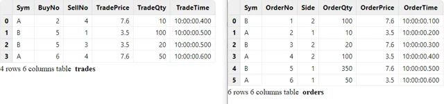
The output table shows that each trade record is joined with its corresponding buy and sell order records from the "orders" stream. It now displays information on the buy and sell quantity, price, and time for each trade.

Window Join: Joining 3-min OHLC with Trades Data
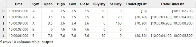
Window joins associate aggregated values from one stream with snapshot records from another.
Here, a 3-minute OHLC bar is joined with all trades that occurred since the previous bar:
// create table
share(table=streamTable(1:0, `Sym`TradeTime`Side`TradeQty,
[SYMBOL, TIME, INT, LONG]), sharedName=`trades)
share(table=streamTable(1:0, `Sym`Time`Open`High`Low`Close,
[SYMBOL, TIME, DOUBLE, DOUBLE, DOUBLE, DOUBLE]), sharedName=`snapshot)
colNames = `Time`Sym`Open`High`Low`Close`BuyQty`SellQty`TradeQtyList`TradeTimeList
colTypes = [TIME, SYMBOL, DOUBLE, DOUBLE, DOUBLE, DOUBLE, LONG, LONG, LONG[], TIME[]]
share(table=streamTable(1:0, colNames, colTypes), sharedName=`output)
go
// create engine
wjMetrics = <[Open, High, Low, Close, sum(iif(Side==1, TradeQty, 0)),
sum(iif(Side==2, TradeQty, 0)), TradeQty, TradeTime]>
fillArray = [00:00:00.000, "", 0, 0, 0, 0, 0, 0, [], []]
wjEngine = createWindowJoinEngine(name="windowJoin", leftTable=snapshot,
rightTable=trades, outputTable=output, window=0:0, metrics=wjMetrics,
matchingColumn=`Sym, timeColumn=`Time`TradeTime, useSystemTime=false, nullFill=fillArray)
// subscribe topic
subscribeTable(tableName="snapshot", actionName="appendLeftStream",
handler=getLeftStream(wjEngine), msgAsTable=true, offset=-1, hash=0)
subscribeTable(tableName="trades", actionName="appendRightStream",
handler=getRightStream(wjEngine), msgAsTable=true, offset=-1, hash=1)
The following script generates mock data and writes trades to the right stream and ohlc to the left stream:
// generate data: ohlc
t1 = table(`A`B`A`B`A`B as Sym, 10:00:00.000+(3 3 6 6 9 9)*1000 as Time, (NULL NULL 3.5 7.6 3.5 7.6) as Open, (3.5 7.6 3.6 7.6 3.6 7.6) as High, (3.5 7.6 3.5 7.6 3.4 7.5) as Low, (3.5 7.6 3.5 7.6 3.6 7.5) as Close)
// generate data: trade
t2 = table(`A`A`B`A`B`B`A`B`A`A as Sym, 10:00:02.000+(1..10)*700 as TradeTime,  (1 2 1 1 1 1 2 1 2 2) as Side, (1..10) * 10 as TradeQty)
// input data
trades.append!(t2)
ohlc.append!(t1)
The correspondence of records between the input streams is shown below:
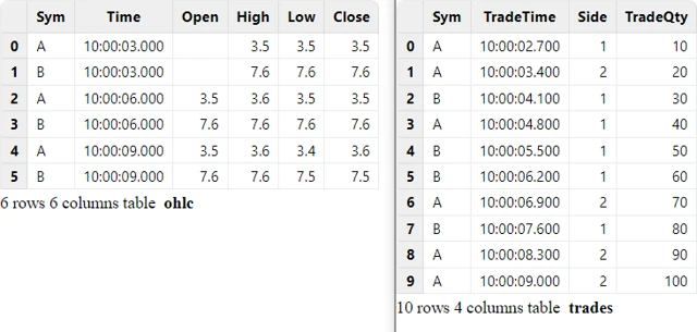
The output table is shown below. The last two columns use array vectors to display all values of column TradeQty and TradeTime within the window.
Complex Event Processing: Strategy Logic
The CEP engine enables users to implement a variety of applications, such as trading strategies (e.g., algorithmic strategies, portfolio trading, arbitrage trading), trading risk management (e.g., real-time risk control and meltdown prevention), and trading monitoring (e.g., visualization). The following is an example of how the CEP engine can be used to realize a financial high-frequency trading strategy.
The strategy determines whether to place an order based on the quoted price change and cumulative trading volume for each stock:
- Two real-time factors are calculated for each trade record: the latest quoted price change relative to the lowest quoted price in the past 15 seconds (R), and the cumulative trading volume in the past minute (V).
- When the strategy is launched, thresholds (R0 and V0) are set for each stock. Whenever the real-time factor values are updated, they are checked against the thresholds: if R > R0 and V > V0, an order is triggered to be placed.
- If the order is not filled within 1 minute after it is placed, it will be canceled.
The following script defines a monitor "SimpleShareSearch" to monitor the event "StockTick". When a stock tick is detected, it triggers the processTick(stockTickEvent) function that logs the name and price of each received stock tick.
class StockTick {
    name :: STRING
    price :: FLOAT
    def StockTick(name_, price_){
        name = name_
        price = price_
    }
}
class SimpleShareSearch {
	newTick :: StockTick  // Cache the latest StockTick event
	def SimpleShareSearch(){
		newTick = StockTick("", 0.0)
	}
	def processTick(stockTickEvent)
	def onload() {
		// Listen to StockTick
		addEventListener(handler=processTick, eventType="StockTick", times="all")
	}
	def processTick(stockTickEvent) {
		newTick = stockTickEvent
		str = "StockTick event received name = " + newTick.name +
			" Price = " + newTick.price.string()
		writeLog(str)
	}
}
dummy = table(array(STRING, 0) as eventType, array(BLOB, 0) as blobs)
createCEPEngine(name="simpleMonitor", monitors=<SimpleShareSearch()>,
dummyTable=dummy, eventSchema=[StockTick])
Conclusion: A Unified Foundation for Real-Time Intelligence
Modern data-driven systems increasingly demand more than isolated stream processing—they require tightly integrated pipelines that combine stateful analytics, cross-sectional insights, event correlation, and automated decision-making.
DolphinDB’s streaming engines provide this unified foundation. From window-based capital flow analysis and real-time factor computation to multi-stream joins and complex event detection, the engine framework enables developers to express sophisticated logic declaratively while maintaining microsecond-level performance.
By chaining engines into streaming pipelines, organizations can eliminate unnecessary data movement, reduce operational complexity, and execute multi-stage analytics within a single real-time workflow. This architecture makes DolphinDB well suited for latency-sensitive environments such as quantitative trading, industrial monitoring, and large-scale IoT deployments.