From Raw Data to Trained Models: An ML Journey
As data-driven applications demand faster insights, teams need ML platforms that integrate seamlessly with their data infrastructure. DolphinDB provides a complete machine learning environment—combining built-in algorithms, plugin support for popular libraries, and distributed computing capabilities—all within a unified platform designed for time-series and analytical workloads.
This article walks through the complete ML workflow in DolphinDB: from data ingestion and preprocessing to model training, evaluation, and deployment. We'll explore supervised and unsupervised learning, demonstrate distributed training at scale, and conclude with a production financial case study.
A First Look
Let's begin with a compact, well-understood dataset to focus on the mechanics of a complete ML workflow in DolphinDB before scaling to production scenarios.
We use the wine dataset provided by UCI Machine Learning Repository to train our first random forest classification model.
(1) Data Import
Download the dataset and save it in file <BookDir>/chapter13/wine.data. Import the data into DolphinDB using the loadText function:
wineSchema = table(
    ["Label","Alcohol","MalicAcid","Ash","AlcalinityOfAsh","Magnesium","TotalPhenols",
    "Flavanoids","NonflavanoidPhenols","Proanthocyanins","ColorIntensity","Hue",
    "OD280_OD315","Proline"] as name,
    ["INT","DOUBLE","DOUBLE","DOUBLE","DOUBLE","DOUBLE","DOUBLE","DOUBLE","DOUBLE","DOUBLE",
    "DOUBLE","DOUBLE","DOUBLE","DOUBLE"] as type
)
wine = loadText("<BookDir>/chapter13/wine.data", schema=wineSchema)
(2) Data Preprocessing
DolphinDB’s randomForestClassifier function requires that the classification labels be integers in the range [0, classNum). The labels in the downloaded wine dataset are 1, 2, 3, so we use the following script to update the labels.
update wine set Label = Label - 1Then define function trainTestSplit to split the dataset into training and testing sets with a 7:3 ratio.
def trainTestSplit(x, testRatio) {
    xSize = x.size()
    testSize = xSize * testRatio
    r = (0..(xSize-1)).shuffle()
    return x[r > testSize], x[r <= testSize]
}
wineTrain, wineTest = trainTestSplit(wine, 0.3)
wineTrain.size()    // 124
wineTest.size()     // 54
(3) Random Forest Classification
Perform random forest classification on the training set with function randomForestClassifier. The function has four required parameters:
- ds: The input data source (usually generated using the sqlDS function).
- yColName: The column name of the dependent variable in the data source.
- xColNames: The column names of the dependent variables in the data source.
- numClasses: The number of classes.
model = randomForestClassifier(
    sqlDS(<select * from wineTrain>),
    yColName=`Label,
    xColNames=["Alcohol","MalicAcid","Ash","AlcalinityOfAsh","Magnesium","TotalPhenols",
               "Flavanoids","NonflavanoidPhenols","Proanthocyanins","ColorIntensity","Hue",
               "OD280_OD315","Proline"],
    numClasses=3
)
(4) Prediction and Persistence
To predict test data with the trained model, use predict(model, X). Trained model can be persisted to disk using saveModel, and loaded from disk with loadModel.
// Predict the test set with the trained model
predicted = model.predict(wineTest)
// Examine the prediction accuracy
sum(predicted == wineTest.Label) \ wineTest.size();
// Output: 0.925926
// Persist model to disk
modelPath = "<BookDir>/chapter13/wineModel.bin"
model.saveModel(modelPath)
// Persisted model can be loaded from disk
model = loadModel(modelPath)
Through this example, we can summarize the typical steps for machine learning in DolphinDB: data preprocessing, model building, data prediction, and model persistence.
Exploring Different Learning Approaches
Machine learning tasks can be broadly categorized into two primary types:
- Supervised Learning is a type of machine learning where the model is trained on a labeled dataset (i.e., the target or outcome variable is known). Supervised learning is commonly used for risk assessment, image recognition, predictive analytics and fraud detection. Common supervised learning algorithms include linear regression, logistic regression, decision trees, support vector machines, and neural networks.
- Unsupervised Learning draws inferences from unlabeled datasets, facilitating exploratory data analysis and enabling pattern recognition and predictive modeling. Common algorithms include clustering (e.g., K-means and hierarchical clustering) and dimensionality reduction (e.g., PCA and factor analysis).
In the following sections, we will explore detailed examples of how to implement supervised and unsupervised learning tasks in DolphinDB.
Supervised Learning: XGBoost Classification
Let's explore supervised learning using XGBoost (eXtreme Gradient Boosting), a powerful ensemble method that combines gradient boosting with sophisticated regularization. XGBoost iteratively trains decision trees, with each tree learning from the residuals of its predecessors, leveraging gradient and second-order derivatives to capture complex data relationships.
DolphinDB supports XGBoost through its plugin system, demonstrating how third-party libraries integrate seamlessly into the platform. We will use the xgboost plugin to demonstrate how to perform machine learning with plugins in DolphinDB.
First, download and load the plugin.
// Check available plugins
listRemotePlugins()
// Install xgboost plugin
pluginPath=installPlugin("xgboos")
// Load xgboost plugin
loadPlugin(pluginPath)
This example continues to use the wine dataset. We use the method xgboost::train(Y, X, [params], [numBoostRound=10], [xgbModel]) for training. The Label column is used as the target variable Y, and other columns are kept as the feature variables X.
Y = exec Label from wineTrain
X = select Alcohol, MalicAcid, Ash, AlcalinityOfAsh, Magnesium, TotalPhenols, Flavanoids, NonflavanoidPhenols, Proanthocyanins, ColorIntensity, Hue, OD280_OD315, Proline from wineTrain
Before training the model, we need to specify a dictionary for params. We will train a multi-classification model so the objective is set to "multi-softmax" and the number of classification num_class is set to 3. You can refer to XGBoost doc for the parameter descriptions.
params = {
    objective: "multi:softmax",
    num_class: 3,
    max_depth: 5,
    eta: 0.1,
    subsample: 0.9
}
Train the model, predict and calculate the classification accuracy:
model = xgboost::train(Y, X, params)
testX = select
          Alcohol, MalicAcid, Ash, AlcalinityOfAsh, Magnesium, TotalPhenols, Flavanoids,
          NonflavanoidPhenols, Proanthocyanins, ColorIntensity, Hue, OD280_OD315, Proline
        from wineTest
predicted = xgboost::predict(model, testX)
sum(predicted == wineTest.Label) \ wineTest.size()
// Output: 0.981481
Unsupervised Learning: Principal Component Analysis
Now let's examine unsupervised learning through Principal Component Analysis (PCA), a dimensionality reduction technique that transforms high-dimensional data into a lower-dimensional space while preserving maximum variance.
This example continues to use the wine dataset which contains 13 dependent variables. By calling the pca function on the data source, the variance weights of each principal component are observed. Set the normalize parameter to true to normalize the data before performing PCA.
xColNames = ["Alcohol","MalicAcid","Ash","AlcalinityOfAsh","Magnesium","TotalPhenols",
             "Flavanoids","NonflavanoidPhenols","Proanthocyanins","ColorIntensity",
             "Hue","OD280_OD315","Proline"]
pcaRes = pca(
    sqlDS(<select * from wineTrain>),
    colNames=xColNames,
    normalize=true
)
The return value is a dictionary. By examining the key explainedVarianceRatio, we can observe that the variance weights of the first three components are very large. Reducing the dimensionality to three components already satisfies training purposes.
pcaRes.explainedVarianceRatio
// Example of returned value
[0.36323402857152510000, 0.18771848509508074000, 0.12316385915570298000,
 0.07144252356377070000, 0.06326142019821392000, 0.05028921085649680000,
 0.04013132045524557500, 0.02834181334036972200, 0.01921589662106918500,
 0.01712296710066611700, 0.01626262987589351800, 0.01216671308985361300,
 0.00764913207611210000]
Keep only the first three principal components:
components = pcaRes.components.transpose()[:3]Apply the PCA matrix to the input data set and call randomForestClassifier for training.
def principalComponents(t, components, yColName, xColNames) {
    res = matrix(t[xColNames]).dot(components).table()
    res[yColName] = t[yColName]
    return res
}
ds = sqlDS(<select * from wineTrain>)
ds.transDS!(principalComponents{, components, `Label, xColNames})
model = randomForestClassifier(ds, yColName=`Label, xColNames=`col0`col1`col2, numClasses=3)
The principal components of the test set also need to be extracted for prediction.
model.predict(wineTest.principalComponents(components, `Label, xColNames))Distributed Machine Learning at Scale
Unlike conventional machine learning libraries, DolphinDB is purpose-built for distributed computing environments, offering a comprehensive suite of machine learning algorithms optimized for large-scale data processing. The core strength lies in its ability to seamlessly execute machine learning algorithms across distributed databases, enabling efficient model training and analysis on massive datasets.
This section demonstrates DolphinDB's distributed capabilities by exploring a use case of logistic regression model training. The following script creates a distributed database partitioned by stock symbols, storing daily OHLC (Open, High, Low, Close) data for each stock from 2010 to 2018.
tickerNo = 3
dateNo = 3287
n = tickerNo * dateNo
ticker = `GOOG`AAPL`MSFT
dates = 2010.01.01..2018.12.31
open = rand(100.0, n)
high = rand(100.0, n)
low = rand(100.0, n)
close = rand(100.0, n)
tickers = take(ticker, n)
dates = stretch(dates, n)
t = table(tickers, dates, open, high, low, close)
dbName = "dfs://trades"
tbName = "ohlc"
db = database(dbName, VALUE, `GOOG`AAPL`MSFT, engine='TSDB')
pt = db.createPartitionedTable(t, "ohlc", "tickers", , `tickers`dates)
pt.append!(t)
The following variables as used as predictors:
- Open/High/Low/Close prices
- Difference between today's open price and the previous day's close price
- Difference between today's open price and the previous day's open price
- 10-day moving average
- Correlation coefficient
- Relative Strength Index (RSI)
The target variable is whether the next day's close price is higher than the current day's close price.
The following preprocessing script defines the calculation logic for these indicators: The function ffill forward fills nulls. The method rsi of the ta module calculates RSI. As calculating 10-day moving average would generate 10 empty rows at first, the first 10 rows are discarded in return.
use ta
def preprocess(t) {
    ohlc = select
             ffill(Open) as Open, ffill(High) as High, ffill(Low) as Low,
             ffill(Close) as Close
           from t
    update ohlc set
      OpenClose = Open - prev(Close), OpenOpen = Open - prev(Open),
      S_10 = mavg(Close, 10), RSI = ta::rsi(Close, 10),
      Target = iif(next(Close) > Close, 1, 0)
    update ohlc set Corr = mcorr(Close, S_10, 10)
    return ohlc[10:]
}
Then generate data sources with the loaded dataset, and call transDS! to apply preprocess to transform the data sources.
ohlc = database("dfs://trades").loadTable("ohlc")
ds = sqlDS(<select * from ohlc>).transDS!(preprocess)
Next, call the DolphinDB built-in logisticRegression function to train the model. The function has three required parameters:
- ds: The input data source.
- yColName: The name of the dependent variable column.
- xColNames: The names of the independent variable columns.
model = logisticRegression(ds,`Target,`Open`High`Low`Close`OpenClose`OpenOpen`S_10`RSI`Corr)Use the trained model to predict results for a specific stock:
aapl = preprocess(select * from ohlc where tickers = `AAPL)
predicted = model.predict(aapl)
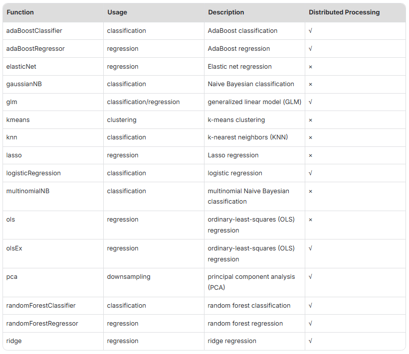
Built-in ML Function Summary
The table below summarizes DolphinDB's built-in machine learning functions and their support for distributed environments.
Financial Application: Stock Volatility Prediction
The previous sections introduced DolphinDB’s machine learning functions and plugins through simple datasets. This section presents a comprehensive machine learning workflow through a feature engineering use case in financial sector.
Volatility measures the degree of price fluctuation within a specific time interval. Inspired by the time series prediction competition Kaggle Optiver Realized Volatility Prediction, we propose a DolphinDB solution covering the data storage, preprocessing, modeling, and real-time volatility prediction for high-frequency market data.
This case uses level-2 quote data to calculate 10-minute indicators as input for predicting stock volatility for the next 10 minutes. A regression model is built using the built-in adaBoostRegressor function. Root mean square percentage error (RMSPE) is used as the evaluation metric, and the trained model achieves a fitting result with RMSPE = 1.729 on the test set.
The features used in this case are as follows:
- Bid-Ask Spread (BAS): The difference between the bid and ask prices.

- Weighted Average Price (WAP): The weighted average price.

- Depth Imbalance (DI): The depth imbalance.

- Press: The buy/sell pressure indicator.




After calculating these metrics, we apply a 10-minute resampling window using group by SecurityID, interval(TradeTime, 10m, "none") to engineer features. The indicator to be predicted is realized volatility (RV), which is computed as the standard deviation of log returns.


Since stock price is not directly available from quote data, we use the weighted average price as a substitute because the actual stock price is typically between the best bid and ask prices. To annualize the volatility, the standard deviation is multiplied by the square root of the number of snapshots in a year.

After data processing, a total of 125,350 records are obtained. We use the following code for train/test split, resulting in 87,744 training and 37,606 test samples.
login("admin", "123456")
dbName = "dfs://sz50VolatilityDataSet"
tbName = "sz50VolatilityDataSet"
dataset = select * from loadTable(dbName, tbName)
            where date(TradeTime) between 2019.01.01 : 2019.06.30
def trainTestSplit(x, testRatio) {
	xSize = x.size()
	testSize = int(xSize * (1-testRatio))
	return x[0 : testSize], x[testSize : xSize]
}
Train, Test = trainTestSplit(dataset, 0.3)
Next, define the evaluation metric RMSPE.

def RMSPE(a,b){
	return sqrt(sum2(1 - b\a)\a.size())
}
Then train the model:
model = adaBoostRegressor(sqlDS(<select * from Train>), yColName=`targetRV,
    xColNames=`BAS`DI0`DI1`DI2`DI3`DI4`Press`RV, numTrees=30, maxDepth=16, loss=`square)
predicted = model.predict(Test)
Test[`predict] = predicted
print("RMSPE=" + RMSPE(Test.targetRV, predicted))
where numTrees specifies the number of trees to generate and maxDepth is the maximum depth of each tree. loss refers to the loss function used for updating sample weights during boosting iterations. Details on other available parameters, such as learningRate and maxFeatures, can be found at User Manual > adaboostRegressor.
Training results:
RMSPE: 1.729
Training Time: 8.6s
We select the stock 600690 as an example to show the volatility prediction from June 25, 2019, to June 30, 2019.
stock_id=`600690
plot((select targetRV,predict from Test
        where SecurityID=stock_id, date(TradeTime) between 2019.06.25 : 2019.06.30),
     title="The realized volatility of "+stock_id,extras={multiYAxes: false})
The red line represents the realized volatility, and the blue line represents the predicted volatility.
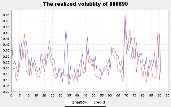
Realized Volatility v.s. Predicted Volatility
Your Complete ML Toolkit in DolphinDB
This article has walked through the complete machine learning lifecycle in DolphinDB—from basic classification tasks to production-grade financial applications. Whether you're building exploratory models on sample datasets or deploying real-time prediction systems on petabyte-scale time series, DolphinDB offers the tools and performance to move from prototype to production efficiently.
Ready to build your next ML application? The patterns demonstrated here—from wine classification to volatility prediction. Start with your data, apply these workflows, and let DolphinDB handle the infrastructure complexity.
Next Steps
To dive deeper into DolphinDB's machine learning capabilities:
- Explore the complete function reference in the User Manual
- Download additional ML plugins with the detailed instruction
- Join the DolphinDB community to share use cases and best practices
- Learn more: https://dolphindb.com/