作者:Yunxia Wang 收听 2 添加反应 Stop Wrestling with Factor Data: A Better Way to Feed Your Deep Learning Models
You've spent weeks fine-tuning your neural network. Your model shows promise in backtests. But when training on real-world factor data, everything grinds to a halt—spending more time loading data than actually training. The bottleneck isn't your model. It's your data pipeline.
In quantitative trading, factor data is exploding: technical indicators, volatility metrics, sentiment scores, alternative data streams. Traditional file-based workflows that once worked now buckle under the weight—CSV files hitting memory limits, pickle dumps clogging storage, data loading becoming the slowest part of your training loop.
This article shows how DolphinDB's AI DataLoader eliminates the data pipeline bottleneck. We'll build a production-ready stock price prediction model, demonstrating how to seamlessly connect database-scale factor data with PyTorch—without the usual memory management headaches.
Challenges of Traditional Approaches
In conventional quantitative strategy development workflows, factor data is typically generated using third-party tools like Python and stored as files. These factors—including technical indicators, volatility metrics, and market sentiment measurements—serve as essential inputs for deep learning models. However, with the rapid expansion of securities trading and the exponential growth of factor data, traditional file-based storage methods expose several critical issues:
- Massive Factor Data Volume: Enormous datasets create substantial pressure on memory bandwidth and storage capacity
- High Integration Complexity: Integrating factor data with deep learning models has become increasingly intricate and resource-intensive
DolphinDB AI DataLoader Solution
AI DataLoader aims to enhance factor data management efficiency and simplify interactions with deep learning models. Specifically, the DDBDataLoader class manages factor data and streamlines integration with deep learning frameworks, creating a more efficient and cohesive workflow. The flow of using DolphinDB data with PyTorch is as follows:
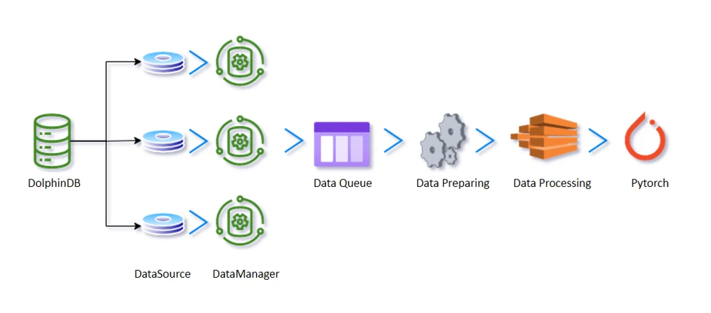
In essence, each DataSource functions as metadata for a partition. A DataSource retrieves data from the DolphinDB server through a session and places the data into a preloaded queue. DataManager processes the data by applying specified sliding window size and step, and transforms it into PyTorch Tensor format.
DDBDataLoader maintains a DataManager pool, with the pool size controlled by the groupPoolSize parameter. Data is extracted from managers by background workers, transformed into appropriate training format, and enqueued for training. DDBDataLoader retrieves processed data from the queue and delivers them to the client for neural network training. This mechanism ensures that only one or a few partitions a are read simultaneously, thus reducing memory consumption.
Practical Case Study: Stock Closing Price Prediction
We'll demonstrate the AI DataLoader's implementation using a practical example. We use 10-minute OHLC data for stock 600690 from January to May 2019 for predicting the next minute's closing price. 1-minute OHLC data from June 2019 serves as our test set for model validation.
Step 1: Data Preprocessing
First, preprocess the dataset to obtain 1-minute OHLC data and save into a DFS table.
data = select TradeTime, SecurityID, first((AskPrice1+BidPrice1)\2) as Open,
        max((AskPrice1+BidPrice1)\2) as High, min((AskPrice1+BidPrice1)\2) as Low,
        last((AskPrice1+BidPrice1)\2) as Close
      from loadTable("dfs://TL_Level2_Snapshot", "SH")
      where date(TradeTime) between 2019.01.01 : 2019.06.30,
          (time(TradeTime) between 09:30:00.000 : 11:29:59.999)  or
          (time(TradeTime) between 13:00:00.000 : 14:56:59.999)
      group by SecurityID, interval(TradeTime, 1m, "none") as TradeTime map
data = data[data.isValid().rowAnd()]
dbName = "dfs://ohlc"
db1 = database("", RANGE, date(2000.01M + til(40) * 12))
db2 = database("", HASH, [SYMBOL, 20])
db = database(dbName, COMPO, [db1,db2], engine='TSDB')
pt = db.createPartitionedTable(table=data, tableName="ohlc_1m",
    partitionColumns=`TradeTime`SecurityID, sortColumns=`SecurityID`TradeTime)
pt.append!(data)
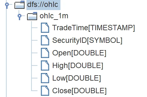
The table schema is structured as follows:
Step 2: Connect to Database and Load Data
Then connect to DolphinDB server through DolphinDB Python API, and use SQL query to load the data in a Python program.
import dolphindb as ddb
from dolphindb_tools.dataloader import DDBDataLoader
from net import SimpleNet # import SimpleNet model from net.py file
import torch
import torch.nn as nn
import time
from tqdm import tqdm
import datetime
import matplotlib.pyplot as plt
import numpy as np
# Connect to DolphinDB
sess = ddb.Session()
sess.connect(ip, port, user, password) # DolphinDB connection info
# Define database and table name
dbPath = "dfs://ohlc"
tbName = "ohlc_1m"
# Set start and end dates
start_date = datetime.date(2019, 1, 1)
end_date = datetime.date(2019, 5, 31)
# Generate list of dates
date_list = [start_date + datetime.timedelta(days=x)
             for x in range((end_date - start_date).days + 1)]
# Format date list
times = [date.strftime("%Y.%m.%d") for date in date_list]
symbols = ["`600690"]
sql = f"""select * from loadTable("{dbPath}", "{tbName}")
            where date(TradeTime) <= 2019.05.31"""
Step 3: Create DDBDataLoader Object
Next, create a DDBDataLoader object using AI DataLoader.
DataLoader = DDBDataLoader(
    sess, sql, targetCol=["Close"], batchSize=64, shuffle=True,
    windowSize=[10, 1], windowStride=[1, 1],
    offset=10,
    repartitionCol="date(TradeTime)", repartitionScheme=times,
    groupCol="SecurityID", groupScheme=symbols,
    inputCol=["Open", "High", "Low", "Close"],
)
Key parameters explained:
- targetCol identifies the column(s) representing the target (dependent variable y) in the training set. Conversely, inputCol represents the column(s) containing the features (independent variables x) used for training.
- windowSize and windowStride define the sliding window parameters. In this configuration, the sliding window size is set to 10 for x and 1 for y, with both utilizing a step size of 1.
- repartitionCol and repartitionScheme are set to further split the query into subqueries. We leverage the previously generated date list to partition the data by trade date, with each subpartition corresponding to a specific date value.
- groupCol specifies the column for data grouping, and groupScheme restricts the filtering range. By setting groupScheme=symbols, the query is limited to data for stock 600690.
Step 4: Build Neural Network Model
After constructing a DDBDataLoader object, we can now build a simple neural network model containing 2 convolutional layers and 2 fully connected layers.
import torch
import torch.nn as nn
class SimpleNet(nn.Module):
    def __init__(self) -> None:
        super(SimpleNet, self).__init__()
        self.channels = [10, 10, 5]
        self.features_in = 20
        self.features_out = 1
        self.conv1d_1 = nn.Conv1d(self.channels[0], self.channels[1], 2, 1, 0)
        self.conv1d_2 = nn.Conv1d(self.channels[1], self.channels[2], 2, 1, 0)
        self.fc1 = nn.Linear(self.channels[2] * 2, self.features_in)
        self.fc2 = nn.Linear(self.features_in, self.features_out)
        self.relu = nn.ReLU()
    def forward(self, x: torch.Tensor):
        x = self.conv1d_1(x)
        x = self.relu(x)
        x = self.conv1d_2(x)
        x = self.relu(x)
        x = x.flatten(start_dim=1)
        x = self.fc1(x)
        x = self.relu(x)
        x = self.fc2(x)
        x = x.reshape([-1, 1, self.features_out])
        return x
Step 5: Model Training
The training loop begins after deep learning model is configured.
# Configure device
if torch.cuda.is_available():
    device = torch.device("cuda")
    print("GPU is available!")
else:
    device = torch.device("cpu")
    print("GPU is not available. Using CPU instead.")
model = SimpleNet()
model.to(device)
# Loss function and optimizer
loss_fn = nn.MSELoss()
loss_fn.to(device)
optimizer = torch.optim.Adam(model.parameters(), lr=0.0001)
num_epochs = 100
# Training loop
model.train()
for epoch in range(num_epochs):
    print("epoch "+str(epoch)+" starts: ")
    begin = time.time()
    for X, y in tqdm(DataLoader):
        y_pred = model(X.to(device).float())
        loss = loss_fn(y_pred, y.to(device).float())
        # print(loss)
        optimizer.zero_grad()
        loss.backward()
        optimizer.step()
    end = time.time()
    print ("epoch "+str(epoch)+" ends, this epoch takes "+
           "{:.2f}".format((end - begin) / 60.0) +" minutes")
Step 6: Model Testing and Result Visualization
Use the following script to make predictions on the test set and display the results with a scatter plot.
symbols = ["`600690"]
sql = f"""select * from loadTable("{dbPath}", "{tbName}") where month(TradeTime)= 2019.06M"""
# Set start and end dates
start_date = datetime.date(2019, 6, 1)
end_date = datetime.date(2019, 6, 30)
# Generate list of dates
date_list = [start_date + datetime.timedelta(days=x) for x in range((end_date - start_date).days + 1)]
# Format date list
times = [date.strftime("%Y.%m.%d") for date in date_list]
# Configure AI DataLoader
dataloader = DDBDataLoader(
    sess, sql, targetCol=["Close"], batchSize=128, shuffle=True,
    windowSize=[10, 1], windowStride=[1, 1],
    offset=10,
    repartitionCol="date(TradeTime)", repartitionScheme=times,
    groupCol="SecurityID", groupScheme=symbols,
    inputCol=["Open", "High", "Low", "Close"],
)
# Make predictions on test data
test_outputs = []
test_targets = []
for inputs, targets in dataloader:
    outputs = model(inputs.float())
    test_outputs.append(outputs.cpu().detach().squeeze(dim=1).numpy())
    test_targets.append(targets.cpu().squeeze(dim=1).numpy())
test_outputs = np.concatenate(test_outputs, axis=0)
test_targets = np.concatenate(test_targets, axis=0)
# Plot the results
plt.figure(figsize=(8, 6))
plt.scatter(test_targets, test_outputs, alpha=0.5)
plt.plot(test_targets, test_targets, color='red', linestyle='--')
plt.xlabel('True Values')
plt.ylabel('Predictions')
plt.title('True Values vs Predictions')
plt.grid(True)
plt.show()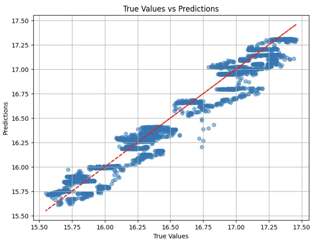
Beyond supporting deep learning training through AI DataLoader, DolphinDB offers Tensor data structures and deep learning model plugins. These tools enable loading trained deep learning models into DolphinDB and executing predictions.
Conclusion
DolphinDB AI DataLoader provides an efficient and flexible data management solution for deep learning applications in quantitative trading. Through this practical case study, we've demonstrated the complete workflow from data preprocessing and model construction to training and testing. The core advantages of AI DataLoader include:
- Memory Efficiency: Controls memory consumption through a partitioning mechanism, effectively handling massive factor datasets
- Seamless Integration: Deep integration with mainstream deep learning frameworks such as PyTorch and TensorFlow
- Flexible Configuration: Supports various parameter configurations including sliding windows and data grouping, adapting to different scenario requirements
Additionally, DolphinDB offers Tensor data structures and deep learning model plugins, supporting the loading of trained models into the database for direct prediction execution, further simplifying the deployment and operations of quantitative trading systems.
For quantitative researchers and algorithmic trading developers, DolphinDB AI DataLoader is undoubtedly a powerful tool for enhancing research and development efficiency and optimizing resource utilization. We hope this article provides valuable reference for your deep learning practices in the field of quantitative trading.
Next Steps
To dive deeper into DolphinDB's deep learning capabilities:
- Explore the complete guide for AI DataLoader
- Download additional Deep Learning (LibTorch) plugins with the detailed instruction
- Join the DolphinDB community to share use cases and best practices
- Learn more: https://dolphindb.com/